With introduction of Dynamic Arrays in Office 365 Excel has one new formula symbol and another that was previously only use in formatted tables.

This article relates to the latest version of Office 365 that has dynamic arrays.

I have previously written about dynamic arrays here.

The new symbol #

Excel has added a new # formula symbol to allow you to easily refer to a spilled range. A spilled range is the output of a dynamic array or a new dynamic array function.

Using the SEQUENCE function from the last blog post, let’s see how we can use the new symbol.

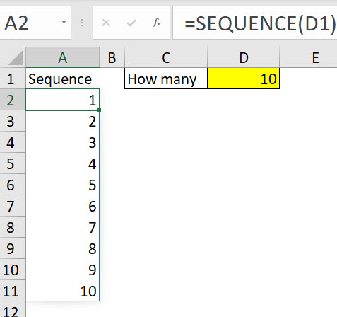
The thin blue line is the spill range for the formula in cell A2. The SEQUENCE function allows you to easily create sequential numbers.

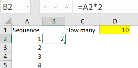
Let’s say we wanted formulas to double those numbers.

We could enter a formula in cell B2 as below and copy it down.

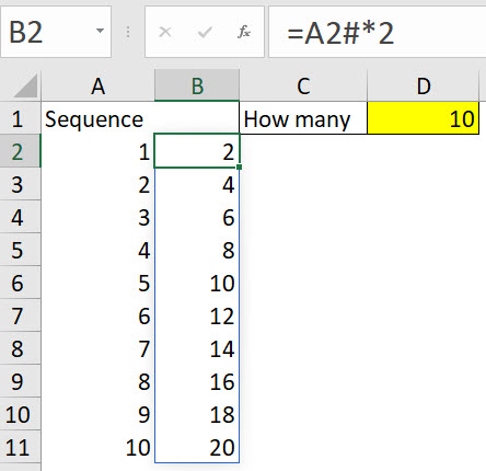
Or dynamic arrays allow us to create a formula that automatically follows the spill range with no copying required. Simply refer to the top left cell of the spill range (the one with the formula in it) and follow the reference with the # symbol as below.

Then as the spill range changes so does the new formula range – see below where we changed cell D1 to 5.

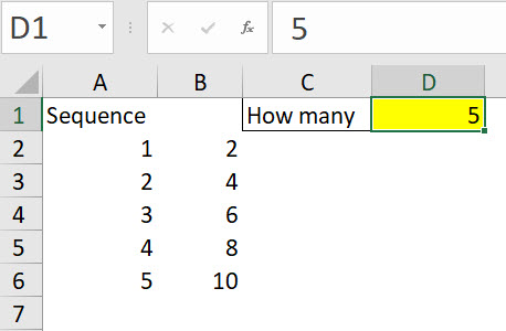
The technique works horizontally, vertically and in a two-dimensional table.

Now let’s examine the other symbol that’s use has been extended.

The extended use symbol @

When you refer to a column on the same row in a formatted table Excel uses the @ symbol – see example below. It basically extracts on the same row, from another column.

In the old Excel there was a technique that involved referring to a range in a single cell. This may have been a range reference or a range name. Either way it is affected in the new Excel.

When you open your old files in the new Excel it may insert the @ symbol in front of some of your formulas or references. See the image below.

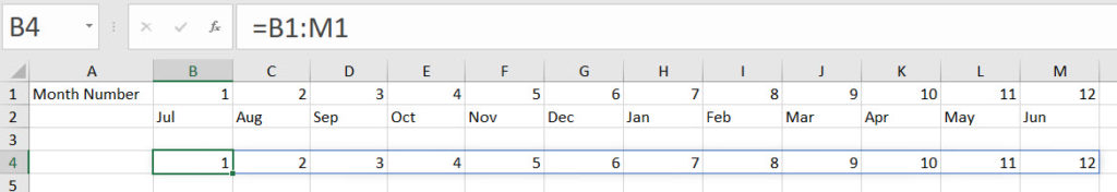
I have entered the following formula in cell B4

=B1:M1

When I hit Enter this will becomes a spill range, even though the range B1:M1 is not a spill range. See below. Note I didn’t need to use $ signs.

In many cases this is exactly what you want to happen. But if it isn’t you can stop it happening.

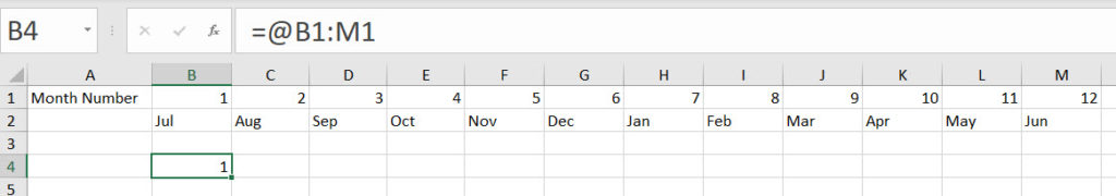
To stop this spill occurring we can use the @ symbol in front of the reference.

=@B1:M1

This says use the reference as you would have in the old Excel and don’t spill the range.

In practice in the old Excel the reference probably would have been a fixed reference as below

=@$B$1:$M$1

Summing up

The # symbol follows the reference and it makes it incredibly easy to refer to spilled ranges. You use the # after the reference to the cell in the top left corner of the spilled range.

The @ symbol precedes the reference and it forces Excel to treat the reference as it would have pre-dynamic arrays.