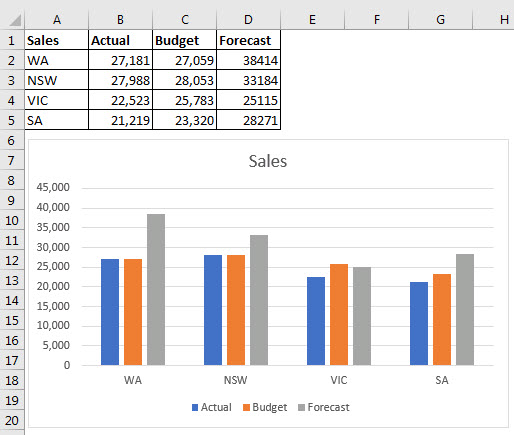
Charts have a behaviour that many people don’t realise. That behaviour can also be turned off. If you hide a row or column in the data range used by a chart, the values will also be hidden on the chart.

That’s the default behaviour. Check out the data table and chart below.

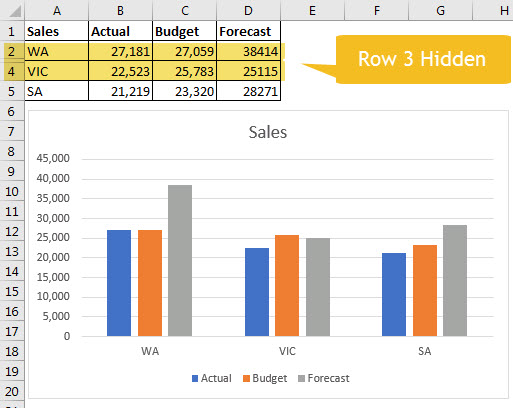
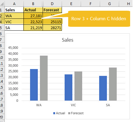
The following two images first hide a row (NSW on row 3). Then a column is hidden Budget (column C). Notice the changes to the chart.

You can use this to your advantage. It doesn’t matter how the cells are hidden.

You can filter the list to hide rows and that will flow through to the chart – see below.

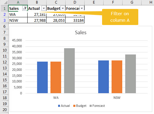
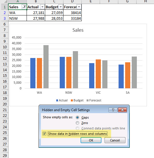
The above chart is based on a filtered list – showing WA and NSW.

Default setting

If you don’t want to hide the results in the chart, you can change the default setting.

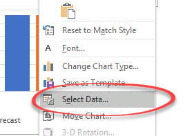
To do that, right click the chart and choose Select Data.

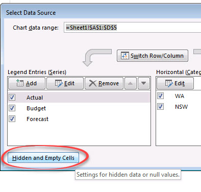
Click the Hidden and Empty Cells button (bottom left corner).

Tick the checkbox for Show data in hidden rows and columns. Click OK.