When I started learning Python, I saw it had a Reverse function and thought, “I could do that in Excel.”

If you want to reverse the characters in a text string or the digits in a number, you could use Excel’s superhero – Flash Fill. This is great if you only need to do it once or twice.

Flash Fill

In the image below I have text in column A and bolded headings in row 1. I have entered the first result that I require in cell B2. This is the structure the Flash Fill works best with.

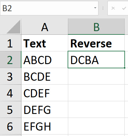
I can now select the range B2:B6 and press Ctrl + E (Flash Fill’s keyboard shortcut). The image shows the result.

If you add extra entries to the list, you must repeat the manual process to update the results.

Custom Function

Flash Fill is great if you only need to do this task a few times. If you need to do it regularly then a custom function is a better solution.

If you are new to custom functions check out this introductory blog post.

Avoid the #DIV/0! Error in Excel

The LET function formula in cell D2 in the image below reverses the text.

This formula captures the text in the txt variable. Then it captures the number of characters using the LEN function in the num variable. The s variable captures a reducing series on numbers that start at character count. The CONCAT function then combines the MID function results. The MID function creates a list of single letters of the txt in reverse order. If txt is empty or blank, it returns a blank cell.      

To test how the custom function will work we can use the LAMBDA function in cell E2.

To create the custom function we create a range name using the LAMBDA function – see image below.

You can see the custom function in action in cell F2, in the image below.