It is best practice in Excel to have a consistent colour for input cells so that users know where they can and need to make changes. You can automate this process by using a Conditional Format.

I typically use a light-yellow background for input cells, sometimes I use the default orange background found in the Styles section on the Home ribbon – see image below.

Instead of applying a format to an input cell you could apply a conditional format that identifies unlocked cells and applies a format to only unlocked cells.

Unlocking

In Excel if you use sheet protection you need to unlock cells that can change – input cells – and then apply sheet protection. All cells are locked as default. Unlocking is not intuitive because it is done via a cell format. In the Format Cells dialog in the Protection tab – see below.

There is a function that identifies locked/unlocked cells. The CELL function has a protect option that returns 1 for a locked cell and 0 for an unlocked cell – see image below.

You can use the CELL function in a conditional format formula to change the cell format is unlocked.

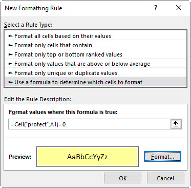
Assuming the range you select include cell A1 the formula to use is

=CELL("protect",A1)=0

See the New Formatting Rule dialog below using the light-yellow fill format.

Changing a protection format will update the cell fill colour.

Check out this previous blog post for a quick way to unlock or lock a cell.