When creating an input range you may need to validate input cells. That may mean ensuring all input cells have an entry. Here’s how.

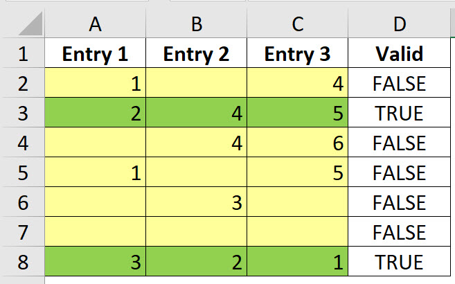
In the image below we need each cell in the three yellow columns on a row to have an entry

Column D displays TRUE when there are three entries and FALSE when there aren’t.

The ever-faithful COUNTIF function does the work here. You can also use COUNTIFS.

The formula in cell D2, which has been copied down is.

=COUNTIF(A2:C2,"")=0

This counts how many blank cells are in the range A2:C2 and compares the count to zero. If there are zero blanks TRUE is displayed. Any other result will return FALSE.

You could use a variation of this formula as part of a Conditional Format to change the input cells green if all three cells have entries.

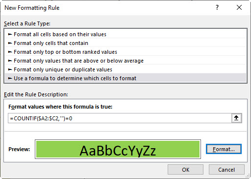
I select the range A2:C8 and clicked the Conditional Formatting icon drop-down on the Home ribbon and selected New Rule.

I select the last option in the top section and entered the following formula.

=COUNTIF($A2:$C2,"")=0

Then I used the Format button and selected a green fill. Then I clicked OK and OK again.

I added an entry on row 3 and you can see the result below.

The important parts of the new formula are the $ signs placed in front of the two column letters.

When you create a formula for use in a Conditional Format you need to create it for the top left cell. But you also need to ensure the formula works for the other cells in the range as well. Hence the $ signs to stop the column references changing.

If you don’t use $ signs the columns will vary in the formulas for the other columns in the range and they will not work as expected. By fixing the column letters you ensure you refer to the correct ranges.