Excel has a Remove Duplicates option in the Data ribbon. It keeps the first item and removes any further items that match.
Monthly Archives: December 2021
Excel Power Query and Data Types
Get the Type right
Data types are an important part of Power Query in Excel and Power BI. They define the type of data that should be in a column. When performing some calculations, getting the column data type right is vital.
Display a New Window
If you have two or more screens (I have three) you can have separate Excel windows on separate screens. This can make copying and linking much easier.
The keyboard shortcut to open a new window in the current file is Alt W N pressed in sequence not held down.
This allows you to have the same file visible in two separate windows. Each window can have a separate sheet.
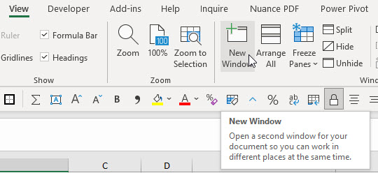
The New Window icon is on the View ribbon tab.
Excel and Emojis
Have some fun with emojis
Yes, you can use emojis (those little images you see in text messages, tweets and posts) in Excel. You can even use them in formulas. ?
Conditional Format to Display Only the First Entry
In my previous blog post I showed a technique to reduce clutter. The technique used a manual formatting method. Here is the automated version.
You can see my previous post here.
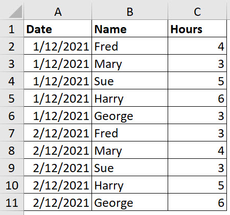
Below is the original table.
We can use a Conditional Format to only display the first entry of each date in the Date column.
Select the range A2:A11.
Click the Conditional Formatting drop down and select New Rule (third from the bottom).
Select the last option in the top section “Use a formula to …”.
In the formula box enter the following formula.
=COUNTIF($A$2:A2,A2)>1
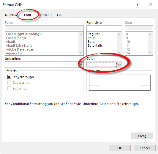
Click the Format button and use the Font tab and change the font colour to White and click OK and then OK again.
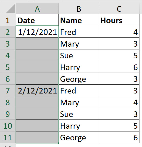
The result is shown below.
The formula for a conditional format must return TRUE to trigger the format. The type of formula that you use is called a logical test, which returns either TRUE or FALSE.
The use of the $ signs is very important in this formula. The COUNTIF function counts the number of entries in a range. If the COUNTIF result is above 1 it is a duplicate. In cell A2 the formula will ALWAYS return 1 as it is counting itself.
When creating a formula-based condition across a range you need to build the formula to refer to the top left cell of the range. In this case we need the range to expand as the range extends down the sheet. Hence, we didn’t use any $ signs on the last two A2 references used.
In cell A3 the formula will be.
=COUNTIF($A$2:A3,A3)>1
This is because the A2 references in the original formula had no $ signs, so they will change with the cell to A3. In our case this COUNTIF will return 2 because the date in cell A3 is a duplicate of the date in A2. This will trigger the format.
This formula expands as the range extends. It uses the cell reference of the cell it is in to determine if the entry is the first entry or a duplicate. This formula will not change the format of the first entry, but it will change the formats of any duplicates.


