The SUBTOTAL function in Excel is quite flexible and in this second post we build an automated summary report using SUBTOTAL.

This is the second post in a series of posts that will look at how we can automate the SUBTOTAL function to summarise a dataset. You can see the first post at the link below.

https://a4accounting.com.au/subtotal-and-dynamic-arrays-in-excel/(opens in a new tab)

Currently our problem is that we can run all 11 functions from the SUBTOTAL, but we don’t know what those values mean. We will need a separate list of function names. Our current layout is shown below.

LET function

We can use the LET function to enable us to combine the labels and the results into a two-column output.

First we need a text listing of the function name labels separated by a character. We can use the TEXTJOIN function to do that based on the existing range.

The formula in cell C19 is.

=TEXTJOIN(",",,C3:C13)

This creates a text string of all the labels in sequence with a comma between each label.

We can then use Paste Special Values to capture the string in a cell. I have pasted it in to cell C21. We will need that string so we can have all the labels in a self-contained formula.

Copy the text string from cell C21. Copy it from the Formula Bar.

The next formula will become quite long but this is a process. We will eventually create a custom function to simplify this.

In cell L3 create this formula.

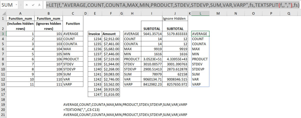
=LET(f,"AVERAGE,COUNT,COUNTA,MAX,MIN,PRODUCT,STDEV,STDEVP,SUM,VAR,VARP",fs,TEXTSPLIT(f,,","),fs)

The LET function allows you to create variables and use those variable names in the formula.

The f variable equals the text string – the string must be enclosed within quotation marks.

The fs variable is a vertical list of those 11 names. The TEXTSPLIT function converts the text string by separating the list using the comma as a delimiter. It creates a vertical list of 11 function names. See image below which displays the vertical list.

We can now expand the formula to include the results of the SUBTOTAL. The new formula for cell L3 is.

=LET(f,"AVERAGE,COUNT,COUNTA,MAX,MIN,PRODUCT,STDEV,STDEVP,SUM,VAR,VARP",fs,TEXTSPLIT(f,,","),sub,SUBTOTAL(SEQUENCE(11),F4:F17),HSTACK(fs,sub))

The sub variable holds the 11 SUBTOTAL results. This was the formula we originally used.

We than use the HSTACK function to combine the two vertical lists in to a single two column table. The labels in the first column and the results in the second column. See image below.

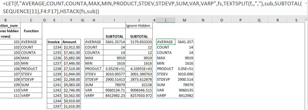
This single formula is spilling across and down to create a summary report on the dataset.

As mentioned, this formula is long and complex. That is a great argument to convert it into a custom function. That is what we will do in the next post.