It is common to have a Factor in a cell or cells in a budget to allow you to easily tweak the numbers by a percentage. If you want to add a Factor to an existing budget model here is how you can do it.

Obviously the examples here are simple but they can be applied to more complex models.

Warning: These changes may not work out as planned so always work on a copy of your model and make sure you are happy with the structure before accepting the changes.

Validations: If your budget/forecast model has validations these changes may affect them and they may need to be tweaked.

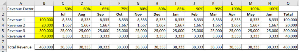
In the image below the yellow cells are input cells.

The before file can downloaded at the button below. The after file can be downloaded at the button at the bottom of the post.

Download Before File

Apply a Single Factor

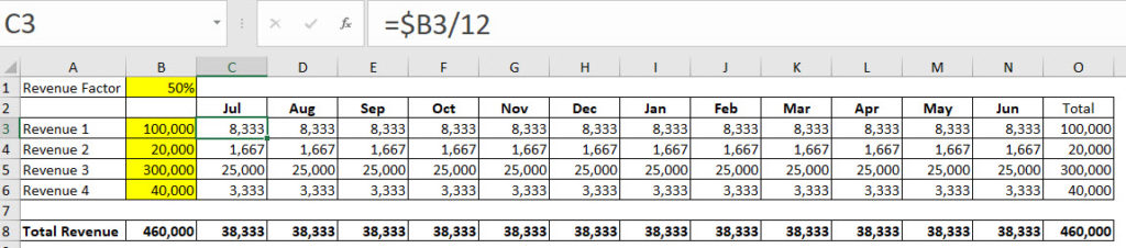
We want to apply a Factor to cells C3:N6 in the allocated months.

The monthly allocation is simple just divide column B by 12 for each month.

The entries in B3:B6 are inputs and are the “normal” sales figures. We need to adjust them for the coming year using the Factor. Rather than change the input cells we want to apply a factor to the allocation cells. That way we can apply “what if” scenarios to see what will happen when varying sales by different percentages.

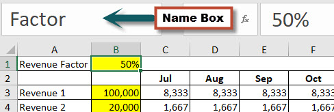
The easiest way to apply a factor is to use a range name.

1. Click cell B1 and click in the Name Box and type Factor and press Enter – see Image below.Note the Name Box on my screen has been increased in size.
2. In a blank cell type =Factor and press Enter.
3. Copy that cell.
4. Select the range C3:N6 and press in sequence Alt  H V S don’t hold the keys down. This opens the Paste Special dialog.
5. Select Formulas and Multiply as per the image below and click OK.
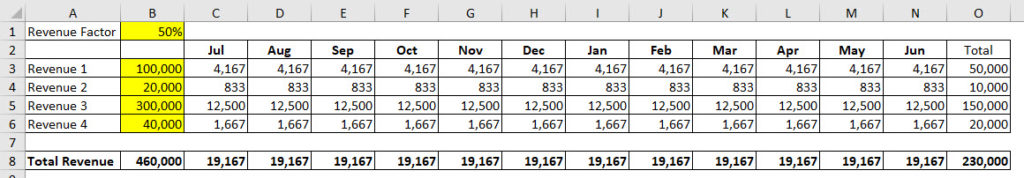
6. That’s it. Changing cell B1 will now affect the allocation calculations. You can delete the entry in the cell you copied.

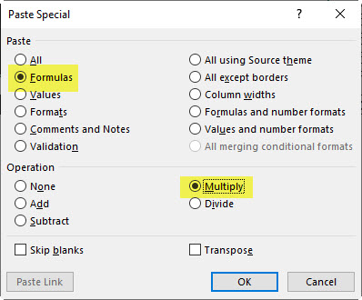
The resulting changes are shown in the image below.

Apply a Range Factor

The above example is simplified as it applies that same percentage across multiple months. If you want to apply varying percentages across the year you can use the same technique with a named range rather than a named cell.

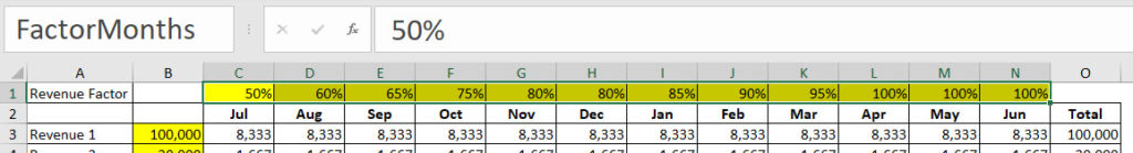
The image below has the structure we will work with.

1. Select the Range C1:N1 and click in the Name Box and type FactorMonths and press Enter. See image below.
2. In cell C10 enter =FactorMonths if you have the latest version of Excel this will automatically copy across to other columns. This is called Spilling and is not what we want. If that happens amend the formula to =@FactorMonths. In the older versions it will just be in one cell.(You can check out this link to learn more about the newer versions of Excel and the Spilling feature.)
3. Copy cell C10.
4. Select the range C3:N6 and press in sequence Alt  H V S don’t hold the keys down to open the Paste Special dialog.
5. Select Formulas and Multiply and click OK.
6. Job done. You can delete the entry in cell C10.

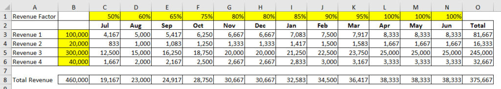
The changes can be seen in the image below

You can download the finished file at the button below.

Download After File