It is common in Excel to calculate the percentage movement or difference between two values. This may be between this year and last year or between actual and budget. There are two common issues you will face when doing this calculation. The first is handling zeros and the second is handling negatives.

In the image below we can see examples of both these issues.

Warning

This simple solution is not meant to handle all cases of percentage comparisons. It handles the situation where you want to identify percentage increases and decrease between two values to identify a movement trend. The solution also avoids using the IF function.  

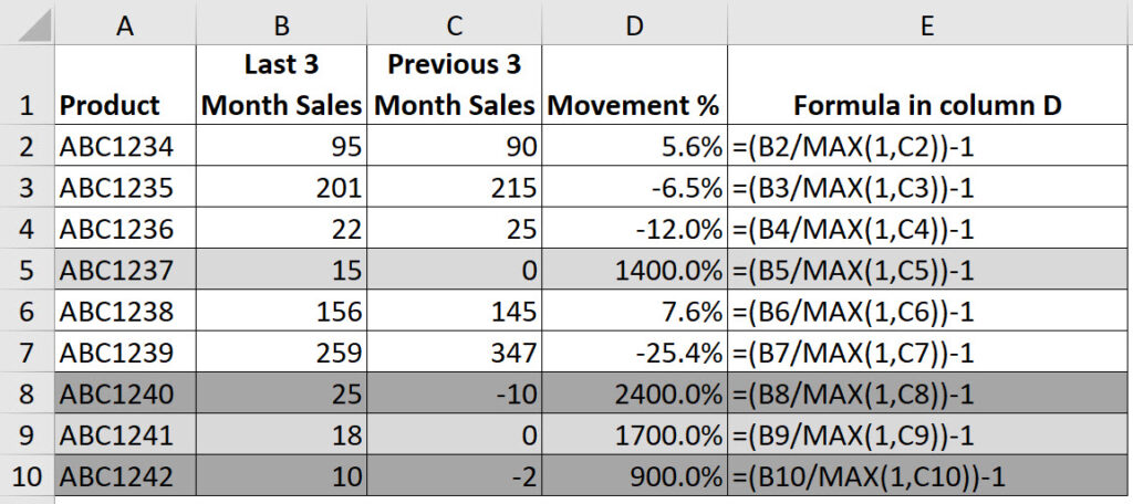
We are comparing unit sales between the last three months (column B) and the three prior months (column C). In column D we want to measure the difference between the two three month periods. We want to identify those products where sales that are increasing, decreasing or relatively static. Column E show the formulas in column D.

Positive percentages in column D mean an increase in sales, and negative percentages mean a decrease.

Identifying the trends can be important when making production or ordering decisions.

This solution is for those type of decisions. It is NOT meant as a solution for all percentage comparisons.

The first three products are straightforward and calculated correctly.

Products ABC1237 and ABC1241 (light grey rows) have zero sales in the previous three month period (column C). This means that even though sales have increased, it is not measured because the divide by zero error is displayed.

Products ABC1240 and ABC1242 (dark grey rows) show the problem when dealing with negatives. These products had negative sales in the previous three months. This causes the percentage movement to be shown as a negative, even though sales increased.

The typical solution to this problem is to use an IF function. But there is an alternative.

MIN/MAX functions

When dealing with zeros and minimum values you can often use the MIN and/or MAX functions instead of the IF function.

In our example we can modify the formula in column D to ensure that instead of dividing by zero or a negative we can divide by 1.

This means that the calculation is not perfect, but for purposes of identifying increasing and decreasing sales it will provide a close approximation of the movement percentage.

In the image below I have amended the formula in column D. I have inserted the MAX function.

MAX(1,C2)

This uses the highest (maximum) value between 1 and C2. If C2 is zero or negative then 1 is used. If C2 is more than zero it’s value is used.

This ensures we divide by one instead of zero or a negative. This avoids the #DIV/0 error and it corrects the negative percentage movement when sales increase, and there is a negative in column C.

As mentioned, this change means that the formulas are not entirely accurate for negatives and zeros. But they now provide a close approximation for the purposes of identifying sales that are increasing or decreasing or static.

Both negatives

If sales in both columns are negative, then this technique doesn’t work.

We are trying to identify increases and decreases in sales. If both values are negative then there have been no sales. There have all been returns or credits.

In the image below I have modified the sales for product ABC1240 and made it -15 in cell B8. I have modified the formula in column D so that it now handles two negative numbers. A negative value in column B is converted to zero.

This means that if both values are negative then -100% is displayed.

Remember this calculation is meant to assist in identifying trends when determining production or ordering requirements based on past sales. It is not a perfect solution but for the purposes of identifying increases and decreases in sales, it does the job without the need to the IF function.