Sometimes Excel refers to columns using numbers. If you need to identify the column letter you can use a few functions in combination. Thanks to Marcus Small for the formula which is shorter and more elegant than my original one. You can also create a custom function.

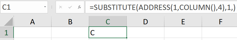
In the image below you can see a formula in cell C1 that returns the column letter for the current cell.

You can download a file with this example using the button at the  bottom of this post.

As you can see this requires the use of three separate functions in combination. We can simplify the use of this combination by including it in a custom function. The formula in cell C1 is.

=SUBSTITUTE(ADDRESS(1,COLUMN(),4),1,)

Two custom functions

One custom function will return the column letter of the current cell. The other will use the current cell as default or allow you to enter a cell reference to return the column from another cell.

Current cell

To use the above function as a custom function we can wrap the LAMBDA function around it and add an extra set of brackets on the end to test it. See image below.

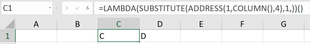
The formula is.

=LAMBDA(SUBSTITUTE(ADDRESS(1,COLUMN(),4),1,))()

We can copy the formula without the extra brackets and paste into a new range name to create a custom function.

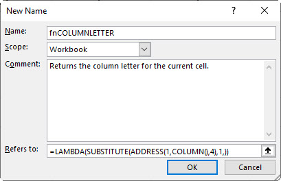
In the Formulas tab click the Define Name icon. In the dialog enter fnCOLUMNLETTER in the name and paste the formula in the Refers to box at the bottom. You can also enter a description in the Comment section – see image below.

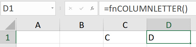
We can now use the function in a cell – see image below.

Column from cell reference

To convert this custom function to accept a cell as input is straightforward.

See the change below where we have added the x variable at the start of the LAMBDA and then used the variable within the COLUMN function brackets.

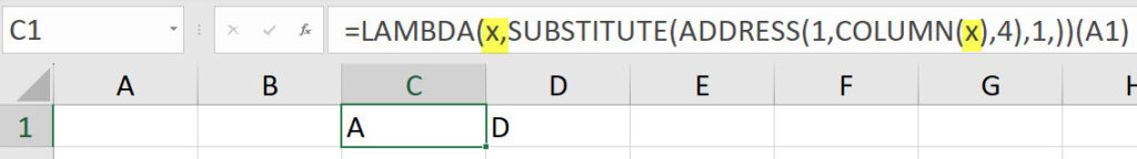
The formula is.

=LAMBDA(x,SUBSTITUTE(ADDRESS(1,COLUMN(x),4),1,))(A1)

Cell A1 (in the brackets on the end) is passed to the x variable at the start of the LAMBDA. In turn x is used in the COLUMN function so that the formula returns the column letter of A.

To enable the function to handle either the current cell or a supplied cell requires a bit more work.

The LAMBDA formula with a cell (top) and without (bottom) is shown in the image below.

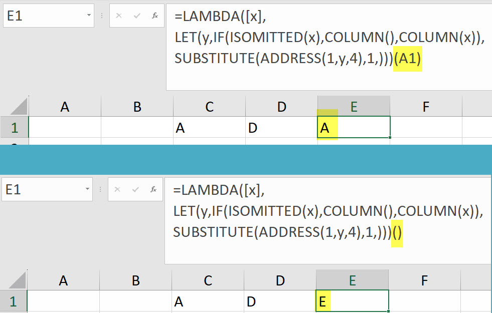
The formula is.

=LAMBDA([x],LET(y,IF(ISOMITTED(x),COLUMN(),COLUMN(x)),SUBSTITUTE(ADDRESS(1,y,4),1,)))(A1)

I have inserted the LET function with a variable y to handle the COLUMN function. The COLUMN function can be used with or without a cell reference.

The y variable is used captures the correct COLUMN function result.

We need to use the ISOMITTED function to identify if the x variable is missing an entry. The ISOMITTED function returns TRUE if the x variable is empty. The IF function uses the ISOMITTED function to decide which COLUMN function result to use.

Note the square brackets around the x variable [x]. This defines the variable as an optional argument. The square brackets syntax for optional arguments is used in Excel’s standard function descriptions.

You can download an example file at the button below.