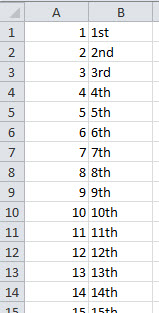
If you need to convert a number to its ordinal so that 1 = 1st and 4 = 4th then there is no built function to do it, but you can write a formula to do it.

The formula is fairly complex so it might be useful to analyse it to understand a few separate techniques that are used together.

The magic formula to convert a number in A1 to its ordinal is

=A1&IF(OR(RIGHT(A1,2)*1={11,12,13}),"th",CHOOSE(MIN(1+RIGHT(A1)*1,5),"th","st","nd","rd","th"))

A link to a file with the formula is at the bottom of the post.

When converting a number to its ordinal there are three rules.

1. Numbers ending in one, two and three have their own unique ordinal “st”, “nd” and “rd” respectively.
2. The exceptions to the first rule are numbers ending in 11,12 and 13 who use the “th” ordinal.
3. Apart from the previous two rules all other numbers use “th”.

So the tricky part is handling numbers ending in one, two or three because of the 11,12 and 13 exception.

As with most exceptions you handle that first in the formula. Let’s look at each part of the formula.

=A1&

The easiest part is the start – this joins the number in A1 to the rest of the formula that figures out the ordinal to use.

IF(OR(RIGHT(A1,2)*1={11,12,13}),"th"

This IF function uses an OR function for the logical test. The OR function examines the result of the RIGHT function.

The RIGHT function extracts the last two characters from A1. The result is multiplied by 1 to convert the text result to a number. That number is then compared to our three exception values.

Using {11,12,13} with the OR function is like creating three separate logical tests within the OR function. The braces { } are associated with array formulas. In this case that are used as a shortened way to refer to more than one value in the OR function.

OR(RIGHT(A1,2)*1={11,12,13})

Is the same as

OR(RIGHT(A1,2)*1=11,RIGHT(A1,2)*1=12,RIGHT(A1,2)*1=13)

but it’s half as long.

Now if any of those tests are true then the IF function returns the “th” ordinal.

The false part of the IF function is a CHOOSE function that handles the remaining numbers.

CHOOSE(MIN(1+RIGHT(A1)*1,5),"th","st","nd","rd","th")

This part of the formula extracts the last digit from A1 using the RIGHT function and multiplies it by one to convert it to a number. If you omit the number of characters from the RIGHT function (as above) it defaults to extracting the last character.

That number has one added to it so that it automatically chooses the correct ordinal.

The first part of a CHOOSE function is a number that chooses an entry from the list of entries that follows separated by commas. See examples below

CHOOSE(1,"th","st","nd","rd","th") will return “th”

CHOOSE(3,"th","st","nd","rd","th") will return “nd”

If a number ends in zero it uses the “th” ordinal. The five ordinal entries listed in the CHOOSE function start with “th” because of zero. That’s why I have to add one to the extracted last number.

I use the MIN function so that 5 is used as the highest value as there are only 5 choices in the CHOOSE function.

So if the last number is zero it will return 1, 1 returns 2, 3 returns 4, 4 or more returns 5.

CHOOSE is a flexible function and can be used in many situations where you need to select from a list of options. It can be simpler to use than multiple IF functions.

Please leave any comments below. If you need more explanation please let me know.

ordinals example file