It is common to have a lot of input cells in an Excel file. It is best practice to use the same format for all the input cells. This makes it easier to identify input cells for you and the user. Here is a technique using Conditional Formats that may be useful.

Let’s take the input cells shown in the image below.

I have used the built-in Input Style for these cells.

As you can see each cell needs a different number format.

Instead of creating a separate Input Styles for each type of input cell, you could use a Conditional Format. You can create your own Styles and copy existing ones, but for this example we can use a Conditional Format to provide the different number formats.

Conditional Format

The text in column B will be used to identify the type of number format to apply in column C.

Select the range C3:C8 and on the Home ribbon tab click the Conditional Formatting drop-down and chose Manage Rules. We use this option because we need to create 6 separate rules, one after the other and Manage Rules enables that more easily.

Click New Rule button (top left).

Click the last option in the top section “Use a formula … “.

In the formula box enter.

=b3="Date"

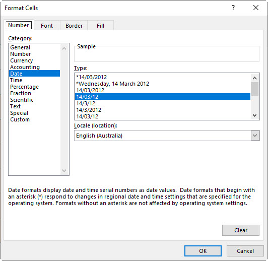
Click the Format button.

Choose the Number tab and select a date format and click OK.

Completed dialog shown below. Click OK to create the Conditional Format.

First one done.

We now need to repeat the process for the other five formats. The final Manage Rules dialog is shown below. Click OK to accept all the rules.

The important part of this technique is that we used the reference to cell B3 in all the formulas. We used B3 because cell C3 was the top, left cell of the range we had selected. The relative position is needed to work for all the other cells.

That means the cell that is looked by the Conditional Format will always be the cell to the left of the format cell.

This means we can use this Conditional Format in any cell provided there is text with the format type in the cell on the left.

See image below where I have copied cell C3 to E11 and entered Percent in cell D11.

Once you have created this Conditional Format you can copy it and use it in other files.

Depending on your sheet structure, you could hide the column that contains the format type as well.