Malcolm Gladwell’s book Outliers is a great read – I reviewed it here. Its premise is that some outliers (events that are far outside “normal” expectations) have causes and hence are worthy of investigation. Excel have some functions that can help identify outliers in your data.
The MIN and MAX functions find the minimum and maximum values in a range respectively. These are straightforward functions that accept a single range or multiple ranges separated by commas. You can also use them in a 3-D calculation on multiple sheets – see blog post to learn about 3-D functions.
Two other functions that I have written about in the past are the SMALL and LARGE functions. They allow you the get the second or third lowest or the second or third highest values in a range – see post here.
Excel 2016 introduced two more functions that can help identify outliers. They are MINIFS and MAXIFS. These work the same as SUMIFS. See this post on how to perform the calculation in Excel 2010 and later versions by hacking the AGGREGATE function. Typically array functions were used before Excel 2010 to do these types of calculations. I tend to avoid using array calculations.
Worked example (file at bottom of post)
Let’s say you get monthly feedback scores per state, per month. You want to identify the highest and lowest scores by state, or by month, or both. The data is on the left and goes further down the sheet. We are extracting the highest and lowest values on the right. The yellow cells are input cells.
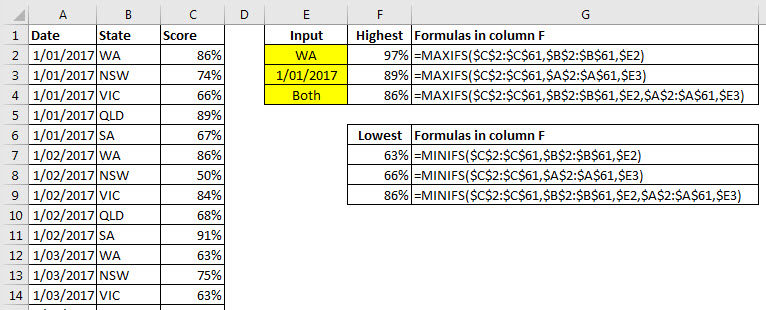
The formulas are shown in column G. These cells use the FORMULATEXT function to display the formulas from column F.
The formula in cell F2 is
=MAXIFS($C$2:$C$61,$B$2:$B$61,$E2)
The first range argument is the range to find the maximum value. The second range argument holds the states to be reviewed. The last argument E2 holds the state entry (WA) to find the maximum value for. Only the cells in column C that correspond to WA entries in column B will be considered when calculating the maximum value.
Cell F3 is based on the date in E2 matching column A. The formula is
=MAXIFS($C$2:$C$61,$A$2:$A$61,$E3)
These are both applying single conditions to the maximum calculation.
Cell F4 has two conditions. Both the state (WA) and date (1/1/2017) must correspond in column B and A respectively to find the maximum value in column C. The formula in cell F4 is
=MAXIFS($C$2:$C$61,$B$2:$B$61,$E2,$A$2:$A$61,$E3)
You can add as many conditions as you want. Each condition requires a range and a condition separated by a comma. You add these two arguments to the right of the MAXIFS function. You need to make sure all the ranges line up eg have the same row numbers – rows 2 to 61 in our case.
You can also use ranges that go across the sheet rather than down the sheet if you need to. In that case the columns in the ranges should line up.
The MINIFS function works in the same way, but performs a minimum calculation.
Please note: I reserve the right to delete comments that are offensive or off-topic.