Recently Liam Bastick (Excel MVP) wrote an article about using the OFFSET function to calculate depreciation in financial models. You can check out the full article here.

When I saw it I wondered if I could use the INDEX function instead of OFFSET.

The OFFSET function is a volatile function which means that it calculates every time Excel calculates, whether it needs to or not. The INDEX function is not volatile. you can download the example file is at the bottom of the post.

These days function volatility is less of an issue as computers are so fast. But I saw it as a challenge to see if INDEX could compete with OFFSET.

I won’t be comparing the techniques, I will just be presenting the INDEX solution. I am not saying this formula is better or worse than Liam’s – just different.

In the image below, the input areas are in yellow. I have split up the capital expenditure (capex) based on the effective life of the assets purchased. The spends in year 7 of $60,000 each are there to show the split of the depreciation in rows 23 to 26.

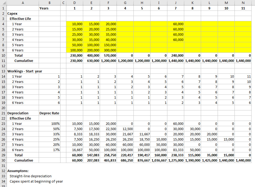
Note the assumptions at the bottom of the image. Straight-line depreciation and the capex is made at the beginning of the year. Also note the effective lives are all full years.

The formulas in row 10 adds up the annual capex. The formula in row 11 add up the cumulative capex over the life of the project.

Workings

The workings section starts at row 13. This determines the start year to use when calculating each category’s annual depreciation.

The numbers represent the first year to use in the depreciation calculation for each Effective Life category. The last year is always the current year.

For a 6 year effective life (row 19) in year 6 you still use year 1 as the start month for the depreciation calculation. In year 7 you use year 2 as the start year – that way you always have 6 years’ worth of capex to add up and depreciate.

The formula for cell D14 which has been copied across and down is

=D$1-MIN(D$1,$B14)+1

The important part of this formula is

MIN(D$1,$B14)

This is similar to what Liam used in his example. This formula uses either the year number (row 1) or the number of years listed in column B. The number of effective years will never be exceeded because we have used the MIN function when comparing the current year and the effective year.

Having used that to determine how many years to use, we then subtract that number from the current year in row 1.

=D$1-MIN(D$1,$B14)

As this potentially deducts the year number from itself to return a zero, we need to add 1 to always at least refer the year 1. Hence the final formula is

=D$1-MIN(D$1,$B14)+1

The INDEX solution

Having figured out the start year to use, we can create a formula to calculate the total relevant capex and multiply that by the relevant depreciation percent.

The formula in D23 is

=$B23*SUM(D4:INDEX($D4:D4,D14))

This has been copied across.

The annual deprecation rate is in cell B23. The SUM function range starts at D4 which is the current year. The end of the sum range is determined by the INDEX function.

Let’s examine the INDEX function in cell K28 and see how it works. In this case the INDEX function is returning a reference to a cell because it is used on the right side of the : symbol.

=$B28*SUM(K9:INDEX($D9:K9,K19))

This works unusually because cell K9 which is at the start of the sum range represents the END of the sum range. The INDEX function below provides the START cell of the sum range. Excel doesn’t care that the cells are entered in reverse. It will add up the range between the two cells.

INDEX($D9:K9,K19)

The entry in cell K19 is 3. This means that INDEX returns the third cell in the range D9:K9 or cell F9 which is the year 3 cell. The sum range works on the range F9:K9 or 6 years’ worth of capex ending in year 8.

Examples

The four 60,000 capex entries in J4:J7 demonstrate the depreciation calculations in isolation in the range J23:M26.

Year 11  

I included Year 11 so you can see there is no depreciation calculated and that the total depreciation (row 30) equals the total capex (row 11) over the life of the project.

Download Example File