The Duplicates option under conditional formatting is useful to identify when there are duplicate entries within a range. This requires you to review the range to see if there are any duplicates. You can use a formula to identify ranges that contain duplicates.
The image below shows the conditional format option that allows you to highlight duplicates within a range.

You can download the example file for this post using the button at the bottom of this post.
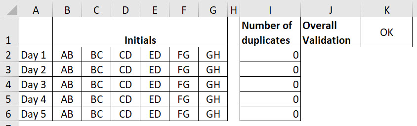
The image below lists days and allocates people’s initials to those days. The conditional formatting is highlighting when I have used a duplicate set of initials.

The problem with this is that you need to actively look at the whole range to figure out if there are any duplicates. This is only a small range, the problem is if the range went down over the page then it would be time-consuming to scroll down each time you wanted to confirm there we no duplicates.
You can use a formula to identify if there are duplicates on a row. Then you can use an overall check to make sure that there are no duplicates in any rows.
The formula in cell I2 is
=SUMPRODUCT((COUNTIF(B2:G2,B2:G2)>1)*1)
This has been copied down the column.
This type of formula is usually only possible when you use an array formula. The SUMPRODUCT function allows you to use array-like formulas without having to enter them as an array.
Note: Excel will soon be releasing a new type of array formula called a dynamic array which will eliminate the need to enter an array using Ctrl + Shift + Enter.
The above SUMPRODUCT function does a conditional count of every entry in the range against the range and compares that to 1. If the conditional count is greater than 1 then TRUE is returned. The TRUE result is multiplied by 1 to convert it into the value of 1. The SUMPRODUCT then adds up all the 1’s to figure out how many rows have duplicates. If the conditional count returned a 1 it means the entry is unique. FALSE would be returned. FALSE is the same as zero and when multiplied by 1 returns a zero so it won’t be counted.
The formula in cell K1 is
=IF(COUNTIF(I2:I6,">0")>0,"Error","OK")
This formula counts how many entries are greater than zero. It compares the result to zero. If there are any non-zero numbers then Error is displayed otherwise OK is displayed.
This means you only need to check one cell to see if there are any duplicates in the range below.
You can see the results in the image below if there are no duplicates.
Please note: I reserve the right to delete comments that are offensive or off-topic.