Stories are memory aids, instruction manuals and moral compasses.
Aleks Krotoskm, broadcaster, journalist, and social psychologist
Stories are memory aids, instruction manuals and moral compasses.
Aleks Krotoskm, broadcaster, journalist, and social psychologist
Financial Functions Part Two
“This accounting webinar series is one of the best for practical CPD hours. It focuses on things we actually use in our day-to-day work, like Excel models and useful tips, instead of theory or topics we may never touch depending on your area of expertise.
It’s clear, easy to follow, and you come away with skills you can put into practice right away. Highly recommend it for anyone wanting CPD that’s actually helpful.”
10/10
C Walthew
November 2024
Using textboxes by themselves can be a good way to add extra content to a spreadsheet. Combining a text box, an icon and an arrow with some colour may make it even better.
The road to success is always under construction.
Lily Tomlin
A recent project required editing many formulas to insert an IF function to display the NA error in certain circumstances. Here’s how I did it.
You’re never going to kill storytelling, because it’s built into the plan. We come with it.
Margaret Atwood author of The HandMaid’s Tale
Excel has re-badged one of the Calculation Options in the Formulas tab – see below. This is a change relating to the new Python capabilities.
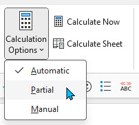
The middle option used to ignore Data Tables (a What If feature on the Data ribbon tab).
The newly named Partial option also ignores Data Tables plus any Python calculations that may take a long time to calculate.
Python calculations are done in the “cloud” and require an internet connection.
Having Actuals, Budget and Variances for each month going across the page is a very common reporting construct. Here is an easy way to sum the correct YTD values as the year progresses.
If you want to automate journal descriptions or create sentences the TEXTJOIN function is your friend. It can combine words and insert the spaces for you.
If you dig a hole and it’s in the wrong place, digging it deeper isn’t going to help.
Seymour Chwast
Source: The Left-Handed Designer
Print ranges can accept dynamic arrays. This means you can set up print ranges that automatically expand or contract based on dynamic array spill ranges.
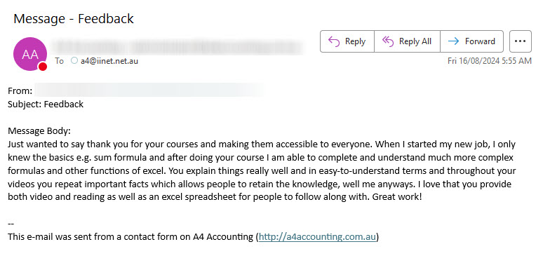
It is always nice to open my email in the morning and receive these types of emails.
I have wished Peter well in his retirement.

I have been using the tbl prefix for my formatted table names in Excel for a long time. There are a few good reasons I use it.
Even if you’re not a teacher, be a teacher. Share your ideas. Don’t take for granted your education. Rejoice in what you learn and spray it.
Source: 9 Life lessons
Tim Minchin
You can select a formatted table when you have a cell or range selected in the table by pressing Ctr + A. But that shortcut won’t work when creating a formula that refers to a formatted table.
To select the table in a formula you must click a cell in the table and press Ctrl + Shift + Spacebar.

I frequently use the shortcut Ctr + ; to enter today’s date in a cell. I thought it would be useful to be able to enter yesterday’s date in a cell. I wrote a one-line macro to do it for me.
Hyperlinks in Excel are a great way to navigate around a file, but they can be easily broken. Try this solution using a formula to create a hyperlink that doesn’t break so easily.
In the image below there is a formula in cell C3 that creates a hyperlink to cell A1.
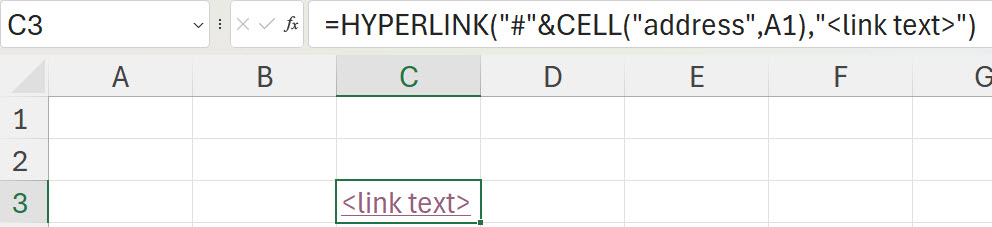
Here is the formula.
=HYPERLINK("#"&CELL("address",A1),"<link text>")Simply change the cell reference from A1 to whatever cell you want to link to. This works for cell in the current sheet.
Hyperlinks to other sheets
In the image below is an example of a link to another sheet.
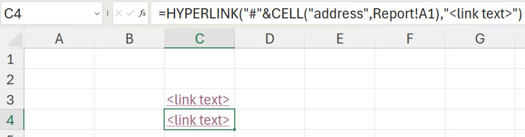
The formula is.
=HYPERLINK("#"&CELL("address",Report!A1),"<link text>")Again, change the reference to create a hyperlink that doesn’t break if the sheet name changes.
Pro Tip
To return after following a hyperlink press in sequence, function key F5 and then press Enter. Don’t hold them down just press F5 then press Enter.

When joining parts of names together, you may want vary the characters you use to separate the name. Depending on the effect you may be able to use array syntax to control the characters and their location.
It is impossible to get better and look good at the same time. Give yourself permission to be a beginner.
Julia Cameron, the Artist’s Way
Style—to renounce all but the essential, so that the essential may speak.
Freya Stark – travel writer
If you need to have a drop-down list automatically adjust and remove items as they are selected, here’s one technique.
Array syntax is a powerful feature in Excel. Array syntax allows you to create a list within your formulas which makes them self-contained. Typing array syntax is difficult as you need to use a combination of quotation marks, commas or semi-colons plus braces (curly brackets).
“Retreating with enthusiasm is a sign of wisdom and long-term thinking.”
Seth Godin
I recently saw a post on LinkedIn about making a drop-down list for a hyperlink interface. It was using a range name and the ADDRESS function. I thought I could streamline it with just the CELL function.
“We first make our habits, and then our habits make us.”
John Dryden
Excel has functions to count the number of rows and columns in a range. It doesn’t have a function to count the number of cells in a range. We can still perform the calculation with the COUNTA function.
It was a nice start to the day to receive this email this morning.
“Doth thou love life? Then do not squander time, for that is the stuff life is made of.”
Benjamin Franklin
I recently saw a post of LinkedIn (from Patryk Samborski) that used the percentage symbol with the SEQUENCE function to produce a list of decimals and I thought I would have a play with that idea.
“It is not how much we have, but how much we enjoy, that makes happiness.”
Charles Spurgeon