The SEQUENCE function returns sequential numbers. Let’s see how we can use it to create a Calendar matrix.

This is the second in a three-part series on using the SEQUENCE function with dates.

You can review the first post here.

You can download the example file at the button on the bottom of this post.

NOTE: The SEQUENCE function is part of the Dynamic Arrays update that is only currently available in the subscription version of Excel.

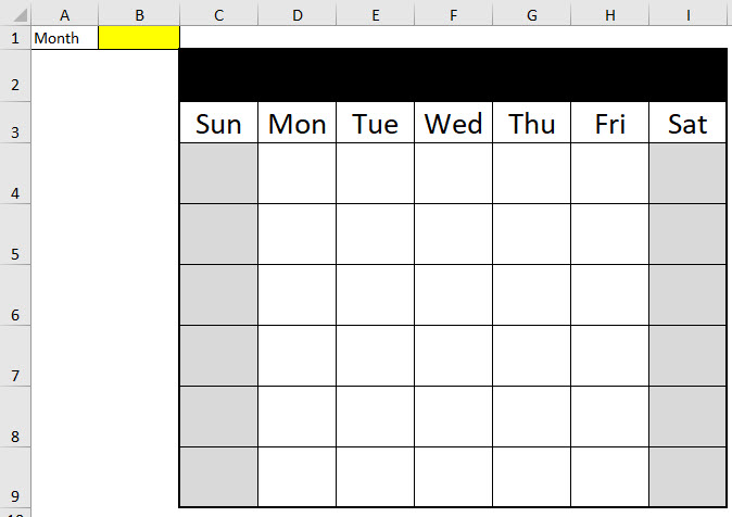
We want to create a Calendar listing as per the image below.

We want to enter a date (the first of the month) in cell B1 and have the calendar created in the matrix below.

Prior to Dynamic Arrays this was possible with a complex array formula. It is easier using Dynamic Arrays.

Before we look at the final solution, let’s see how the SEQUENCE function works in a matrix.

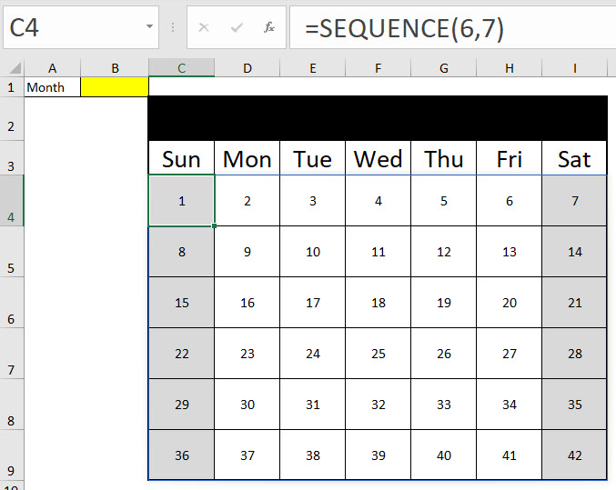
In cell C4 is enter the following formula.

=SEQUENCE(6,7)

The result is shown below.

The 6 represents the number of rows to populate and the 7 the number of columns to populate. The default settings for SEQUENCE starts at 1 and increments by 1 – precisely what we need.

We can use this SEQUENCE function with other functions to create a matrix listing of dates for a specific month.

Sunday start

In general there are two ways to display a Calendar.

1. Start on a Sunday
2. Start on a Monday.

I prefer the Monday start, but let’s look at the Sunday start first.

The title formula used in the image below in cell C2 is

=TEXT(B1,"mmmm yyyy")

This shows the full month name and I have used the Center Across Selection format.

The formula for cell C4 is

=IF(MONTH(B1+SEQUENCE(6,7)-WEEKDAY(B1))=MONTH(B1),DAY(B1+SEQUENCE(6,7)-WEEKDAY(B1)),"")

The result is shown below.

Let’s review the parts of the formula.

The part that does all the hard work is

B1+SEQUENCE(6,7)-WEEKDAY(B1)

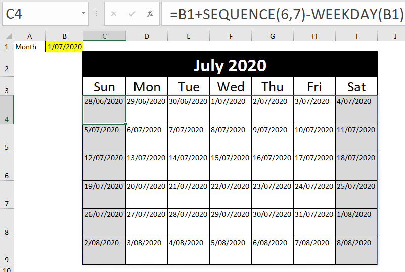
This populates the matrix with dates. If I enter that formula into cell C4

=B1+SEQUENCE(6,7)-WEEKDAY(B1)

You can see the result below.

As you can see this includes the dates both before and after the month we want.

The WEEKDAY function returns a number for 1 to 7 representing the day of the week. Sunday is 1 and Saturday is 7. This function helps us match the correct date to the correct day of the week for each column.

The columns starts on Sunday. Sunday is represented by 1 in the WEEKDAY function.

We don’t know the date entered in cell B1. It needs to be the first of the month. To make sure that the date is displayed in the correct column we add the SEQUENCE number and then deduct the WEEKDAY number.

In cell F4 the calculation goes like this

Start with 1/7/2020 from B1 and add 4 from the SEQUENCE function (it is the fourth cell in the range) and then deduct the weekday number for 1/7/2020 which also happens to be a 4 because it is a Wednesday. So 1/7/2020 is displayed in cell F4.

Let’s look at the calculation cell H4.

Start with 1/7/2020 from B1 and add 6 from the SEQUENCE function (it is the sixth cell in the range) and then deduct the weekday number for 1/7/2020 which is 4 because it is a Wednesday. So 3/7/2020 (1/7/2020 + 6 – 4) is displayed in cell F4.

Each column has the same adjustment based on the WEEKDAY value of the date in cell B1.

Every cell is first incremented by the SEQUENCE number and then the WEEKDAY value of cell B1 is deducted. This aligns the dates with the correct day column.

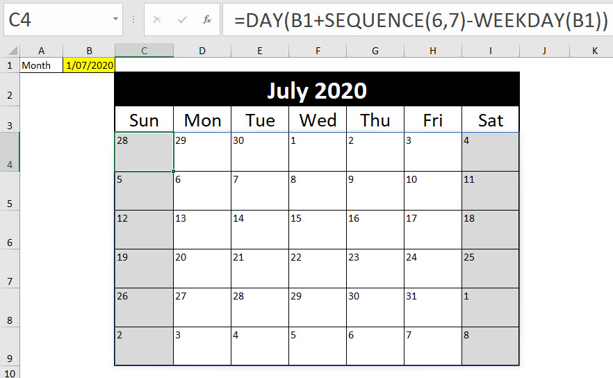
We don’t want to display the date in the matrix, we want to display the day number. We add the DAY function in cell C4 – see image below.

=DAY(B1+SEQUENCE(6,7)-WEEKDAY(B1))

The DAY function returns the day number from the date.

For our purposes we need to remove all the dates that aren’t part of our month. We need to add the IF function to the start and compare the month number from the our calculated date to the month number of the date in cell B1.

If the month numbers match, we display the day. If they don’t, we display a blank cell using the “”.

Monday start

To create a Calendar matrix for a Monday start you only need to change the formula slightly.

We can amend the WEEKDAY function to return 1 for Monday instead of Sunday. Then Monday = 1 and Sunday =7. To make that change you add ,2 to the end of the WEEKDAY function.

The formula for a Monday start in cell C4 is

=IFERROR(IF(MONTH(B1+SEQUENCE(6,7)-WEEKDAY(B1,2))=MONTH(B1),DAY(B1+SEQUENCE(6,7)-WEEKDAY(B1,2)),""),"")

The result is shown below. The two formula changes are highlighted in yellow in the Formula Bar.

I have used a grey format to show the weekends.

What if you want to highlight holidays as well?

That’s what we will cover in the next post.

Download Example File