The SEQUENCE function returns sequential numbers. Let’s see how we can use it with a list of dates.

This is the first is a three-part series on using the SEQUENCE function with dates.

If we need a list of dates in a specific month, we can create a single formula to create the list using the new SEQUENCE function.

NOTE: The SEQUENCE function is part of the Dynamic Arrays update that is only currently available in the subscription version of Excel.

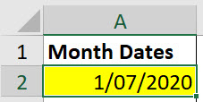
In the image below we want to create a list of dates for the month starting from 1/7/2020 (July 1 2020).

In cell A3 we can use the following formula

=IF(MONTH(A2+SEQUENCE(30))=MONTH(A2),A2+SEQUENCE(30),"")

A more elegant solution was suggested in the comments – I have included it at the bottom of the post.

This creates the following list.

Things to Note

• Notice the thin blue line around the range A3:A32. This is called the “Spill” range and is part of the Dynamic Array functionality.
• In this case the Spill range varies based on the number used in the SEQUENCE function.
• Cell A4 doesn’t not contain a formula – the only cell that has a formula is cell A3. The top, left cell in the Spill range contains the formula.
• At the moment the Spill range does not copy formats from the first cell. I have manually formatted the range as a date.
• None of the cell references used $ signs. Dynamic Arrays reduce the need to use $ signs in cell and range references.

Let’s examine a part of the formula.

A2+SEQUENCE(30)

This is the part of the formula that does all the work. SEQUENCE(30) provides a vertical list of 30 numbers from 1 to 30.

For July that is all we need because July has 31 days. The months that don’t have 31 days will list the next month’s dates at the bottom of the list – not what we want.

To handle months with less than 31 days we need to add the IF function.

The IF function checks to make sure the month number of the date we create is the same as the month number of the date in cell A2. If it isn’t, a blank cell is displayed.

Using “” is how you tell Excel to display a blank cell.

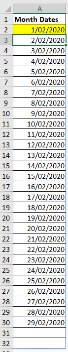
The image below shows the result for February 2020. Notice that the Spill range includes blank cells at the bottom.

In future posts I will cover how to create a Calendar listing of dates for a month (rows and columns) using a single formula.

Added 21 July 2020

The more elegant solution is

=IFERROR(SEQUENCE(EOMONTH(A2,0)-A2)+A2,"")

This uses the EOMONTH function to find the end of the month and deducts the start date to figure out how many days need to be added. This is what the SEQUENCE uses to then add to the date.

Thanks Consensure for sharing in the comments.