I covered a solution to sorting and ignoring the sign a couple of years back, but it is time to revisit this thanks to dynamic arrays.

The problem was someone wanted to sort a list based on values, but ignore the value’s sign. So -44 is next to 44.

The original solution involved a helper column with the ABS function – you can read the blog here.

Dynamic arrays

The subscription version of Excel has dynamic arrays. They offer the ability, in some cases, to remove the need for helper cells.

Helper cells are extra cells that make the final formula easier to create, shorter or simpler.

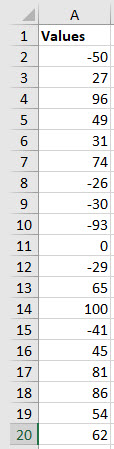
Below is the list we want to sort.

In cell C2 we can use the following formula to achieve our sign-less sort.

=SORTBY(A2:A20,ABS(A2:A20))

See the result below.

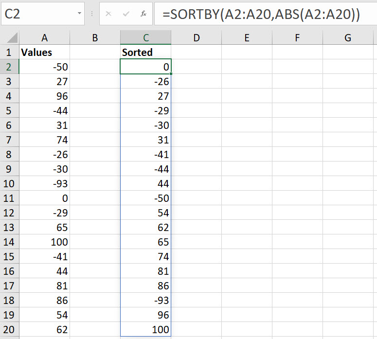
Wrapping the range within the ABS function creates a range in memory that has all the positive numbers. The ABS function removes the negative sign. These positive values are then used in the SORTBY function to do the sort of the original range.

This has the advantage of leaving the original range unchanged and having a separate, sorted list.

The formula is only in cell C2 and it spills down. Spilling is part of the dynamic array functionality. I have covered dynamic arrays in previous posts. See this one as a start.