This post is inspired by the book 101 Ready-to-Use Excel Formulas by Michael Alexander and Dick Kusleika. Formula #10 allows rounding to a certain number of significant digits. This post shows how to convert that formula into a custom function.
OK, what are significant digits? I must admit I had forgotten about them from high school Maths class. They relate to how many digits you want to show to measure a large value. So, a number like 654,321 rounded to 2 significant digits is 650,000.
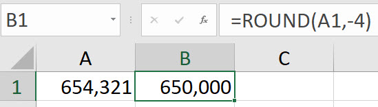
The ROUND function can round to the left of the decimal point using negative numbers. The problem is the negative number you need to use is determined by how many total digits are in the number you want to round. In the example above you would use -4 – see image below.
The book had a formula that determines this number, so it isn’t hard-keyed into the formula – see image below.

The +2 on the end is how many significant digits to round to. Changing that number changes how many significant digits. Here is the formula.
=ROUND(A2,LEN(INT(ABS(A2)))*-1+2)
Custom function
Whenever I see more than two functions nested, or used together, I immediately think about creating a custom function to simplify the calculation and make it easier to use and understand.
Here is the LAMBDA function formula to test.

Here is the formula.
=LAMBDA(amt,digits,ROUND(amt,LEN(INT(ABS(amt)))*-1+digits))(A3,2)
If you are new to LAMBDA custom functions check out the post below.
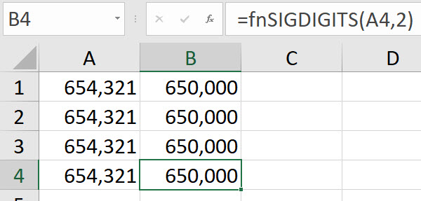
The custom function in operation is shown below.
The New Name dialog for the custom function is shown below.
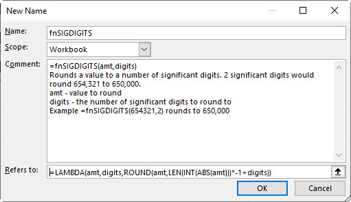
I recommend using the Comment section to explain and demonstrate the custom function.
Please note: I reserve the right to delete comments that are offensive or off-topic.