Many of Excel’s functions have default arguments. What are arguments? Arguments are the sections within a function that you separate with commas and some of these arguments are optional.
To discover if an argument is optional, look at the function argument list that pops up when you start to create a function. If a function argument has square brackets around it then it is optional. The optional arguments tend to be on the end of the function arguments.
Example
The LEFT function takes two arguments the second one is optional – see image below.

If you omit the second argument the LEFT function extracts the first character. The num_chars argument defaults to one character if omitted. See image below.

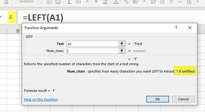
To find out what the default is you can use the Function Arguments dialog (click the fx icon on the Formula Bar) and click the box for the argument. The description will include what the default is. See image below.
Common Default Arguments Omitted
The RIGHT function defaults to one character and extracts the last character when the num-chars argument is omitted.
The VLOOKUP function defaults to the approximate_match argument or TRUE or 1 if the last argument, range_lookup, is omitted. This means the table being looked up needs to be sorted by the left column.
The DOLLAR function defaults to two decimal places if the last argument, decimals, is omitted. This function converts numbers into formatted text dollars numbers using $ and the comma 100 0separator.
The SUMIF function defaults to summing the range_criteria if the sum_range is omitted. This is useful when you are doing criteria like greater than zero or less than zero on a range of values.
When creating functions keep an eye out for the default square brackets.


Please note: I reserve the right to delete comments that are offensive or off-topic.