I recently downloaded an example file for an Excel challenge. The challenge had a lot of things to do but they were all based on a Timestamp column that had text instead of times.

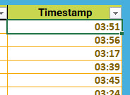
The top of the challenge file is shown in the image below.

The value in cell F14 shows that it is text. It looks like a formatted time but it is text. This means Excel won’t be able to work with this entry as a real time value. I also removed the alignment format from the column and you can see the text is left aligned. This is another clue that Excel treats it as text. Numbers, dates and times are right aligned.

The idea of the challenge was, I imagine, to get the correct answer in the shortest time. So the best solution would be the quickest, as the whole challenge hangs on the entries in the Timestamp column being real times.

Quickest solution

Since this is a one-off challenge, I would use the following technique.

1. Click cell F14 and press Ctrl + Shift + down arrow. This selects the whole column to the bottom. Luckily there are no blanks in the column.
2. Press Ctrl + H.
3. Type h in the top box and click the Replace All button.
4. Type m in the top box and click the Replace All button.
5. Type s in the top box and click the Replace All button.
6. Press Ctrl + 1 and use the Custom Number Format mm:ss and click OK.

Job done. This takes surprisingly little time – the result is shown below.

Other solutions

The above solution was quick, but it was manual. If time wasn’t an issue (pardon the pun) and the Timestamp column data needed to be regularly converted, you could use a formula or Power Query to do the conversion.

Formula solution

The formula that converts the text entries in column F into real times is.

=TIME(LEFT(F14,2),MID(F14,5,2),MID(F14,9,2))

This works because the layout used is a fixed structure. This allows us to key in the position numbers to identify where the digits will be in the string of numbers and text.

One thing to note is that the structure of the TIME function requires numbers for the three arguments hours, minutes and seconds. Both the LEFT and MID functions return text numbers, not real numbers. But the TIME function is accommodating and converts them into numbers for us.

Power Query solution

This may be overkill for a challenge like this, but Power Query is a skill worth learning and practicing.

Here goes.

1. Click a cell in the table and press Ctrl + A – this selects the whole table.
2. Click on the Data ribbon and click the From Table/Range icon (left-hand side).
3. Click OK to accept the table being created.
4. In the Power Query windows that opens right click the Timestamp column and choose Replace Values.
5. In the dialog that opens enter h in the top box and click OK.
6. Right click the Timestamp column and choose Replace Values enter m in the top box and click OK.
7. Right click the Timestamp column and choose Replace Values enter s in the top box and click OK.
8. Click the small icon on the left of the Timestamp header row and select Time.
9. Click Close and Load on the far left of the home ribbon. This creates a totally separate output table with the corrected time.

You may want to format the Timestamp column in the output table using the Custom Number format mm:ss.

To update new data or times from the source table, just right click the output table and choose Refresh.

Conclusion

This example was from a challenge, but as you can see there are usually a few ways to do things in Excel. The one you use is based on how frequently you need to do, or repeat, the task.

Yet another automated solution would have been a macro which I will cover in the next post.