I was looking at a calendar and noticed it used alternately shaded cells, like a checkerboard, for all the dates and thought Excel could do that.

Conditional Formats can be used to apply different formats across ranges based on different conditions.

When you use a Conditional Format it means inserted rows and columns will automatically be adjusted to the format.

The formula I used for the Conditional Format ended up being fairly long and there may be an easier way to do it, but it works.

(31-Aug-2016 – Jason posted a better formula in the comments section and I came up with my own spin on it –  see comments at bottom of post)

(A famous person once wrote  “Sorry this letter is so long. I didn’t have to time to write a short one” – this can relate to formulas as well)

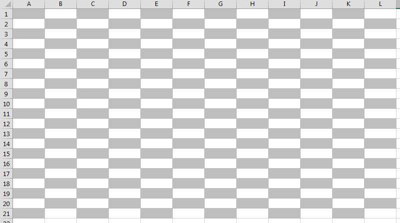
To apply the checkerboard format first select the range to apply it to. I have used A1:L21.

You need to know the first cell in your range as this is the cell you need to include in the formula.

On the Home ribbon click the Conditional Formatting icon drop down and choose New Rule.

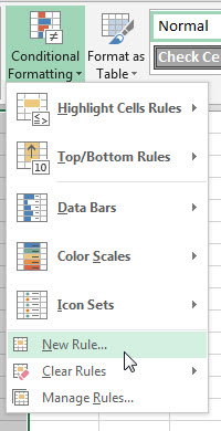
Then select Use a formula to determine which cells to format.

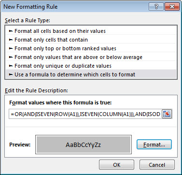
Copy the formula from below and paste in the Formula box and click OK.

=OR(AND(ISEVEN(ROW(A1)),ISEVEN(COLUMN(A1))),AND(ISODD(ROW(A1)),ISODD(COLUMN(A1))))

Click the Format button and click the Fill tab to select a fill colour – I have used a grey.

Click OK again to apply the format.

The formula in the Formula box must return TRUE to trigger the format.

The cell reference in all the functions must be the top left cell of the range selected. It must be relative reference so it cannot contain any $ signs.

Here is the formula again

=OR(AND(ISEVEN(ROW(A1)),ISEVEN(COLUMN(A1))),AND(ISODD(ROW(A1)),ISODD(COLUMN(A1))))

The OR function returns TRUE if any of its arguments returns TRUE.

The two arguments in the OR are both AND functions.

The AND function only returns TRUE if ALL its arguments are TRUE.

The ISEVEN function returns TRUE when the value is even.

The ISODD function returns TRUE when the value is odd.

The ROW function returns the row number of the reference.

The COLUMN function returns the column number of the reference.

The first AND function ensures both the row and column numbers are even.

The second AND function ensures both row and column numbers are odd.

So the rule that is applied by the above formula is

“If both the row and column numbers are even OR if both the row and column numbers are odd then apply the shaded format.”

This rule can be seen from the matrix below.

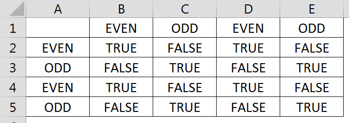
The formula in cell B2 is

=OR(AND(ISEVEN(ROW()),ISEVEN(COLUMN())),AND(ISODD(ROW()),ISODD(COLUMN())))

This has been copied down and across and is the same formula as the conditional format rule, but the references have been removed.

Both the ROW and COLUMN functions can return a result without a reference. If the reference is omitted the function uses the row or column that the formula is in.

The link to the example file is below.

checkerboard file