Who doesn’t get satisfaction from drawing a line through a completed task? That sense of achievement. Well you can do the same in Excel.

Let’s say you have a list of month end tasks. You can download an example file at the bottom of the post.

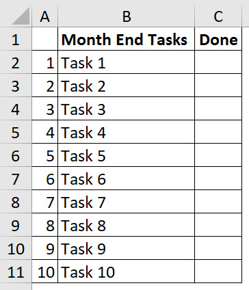
We need to work our way through the tasks. We want to place an x in the column C and have Excel place a line though the task in column B.

A conditional format can do the work for us.

Steps

1. Select the range B2:B11.
2. Click the Conditional Formatting icon on the Home ribbon and select New Rule
3. Select the bottom option in the top section “Use a formula …”
4. In the formula box enter the following formula

   =$C2<>""

   Note: Placement of the $ sign is important. Also the row number shouldn’t have a $ sign so it changes for each cell in the range.

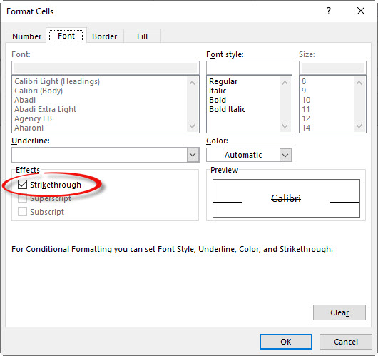
5. Click the Format button and choose the Font tab. Make sure the Strikethrough option is ticked – you might have to click it once or twice to get the tick. Click OK.
6. Click OK again.
7. Enter x or any other character anywhere in the range C2:C11 and column B should automatically update. You must press Enter after you type the entry.

Job done – put a line through it.

Column B will revert back if the entry is removed from column C.

Download Example File