The Australian Financial Year has its challenges. Working out the Quarter number based on a date has a few solutions. Here’s another one.

In the image below we have dates in column A and the financial year quarter in column B. Column C has the calendar year quarter formula.

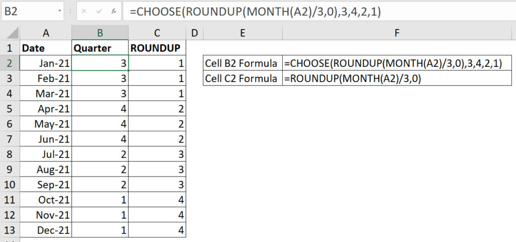
We use the calendar year quarter formula (below) within the financial year quarter formula.

=ROUNDUP(MONTH(A2)/3,0)

The ROUNDUP function round values up to the closest whole number. The MONTH function returns a number from 1 to 12 representing the calendar month number.

We divide the month number by 3 and then round it up to the nearest whole number based on zero decimal places. As an example, April is month 4 and when divided by 3 returns 1.3333. This is rounded up to 2. The month numbers 3, 6, 9 and 12 return whole numbers and are not rounded.

The CHOOSE function allows you specify a number, and based on that number, return from a sequential list of entries.

As an example. The following formula returns the word Pear.

=CHOOSE(2,"Apple","Pear","Orange")

The first argument is 2 which means extract the second entry from the following arguments listed.

The financial year quarter formula in cell B2 is

=CHOOSE(ROUNDUP(MONTH(A2)/3,0),3,4,2,1)

The ROUNDUP function provides the calendar year quarter number. We then provide the 4 numbers that equate to the financial year quarters. It is like mapping the four calendar year quarters to their corresponding financial year quarters.

This post from many months back has another solution.