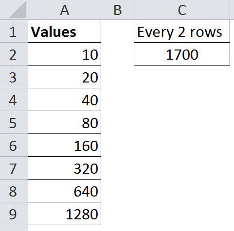
Let’s say you have a list of values that has a set sequence. In the list which starts in row 2 you want to add up every second entry. So you want to add up the entries in row 3, row 5, row 7 etc going down the sheet. The SUMPRODUCT function to the rescue yet again.
The following formula in cell C2 will add up every second row in column A starting at row 3
=SUMPRODUCT((MOD(ROW($A$2:$A$9),2)=1)*($A$2:$A$9))
The MOD function returns the remainder after dividing one number by another. The ROW function provides the row numbers for each cell in the range A2:A9.
The row number is divided by 2 and the MOD returns the remainder. Remainders that equal 1 are the rows we want to add up – they are all the odd numbers. That is because the values start in row 2.
The entries in the odd rows will return TRUE, which in Excel is 1 and the 1’s are multiplied by the corresponding values in the rows and added up by the SUMPRODUCT function.
Even row numbers return FALSE which is the same as zero. Multiplying by zero will zero the values and are hence they are not added up by the SUMPRODUCT function.

Thanks for posting.
I’m having trouble seeing in what circumstances one would want to add every other row. Does anyone have real life examples?
You would use this type of formula if there was a report that had a strict format that didn’t allow you to conditionally add up the rows any other way.
It is also an example of using functions within the SUMPRODUCT function. Normally this calculation is done with an array formula.
The formula can be easily amended to add up every third, or fourth row as well.
Regards
Neale