If you have two lists of numbers and you need to ensure they are identical there is a simple formula that can confirm they match.

This assumes that the values are next to each other in a table layout. See image below.

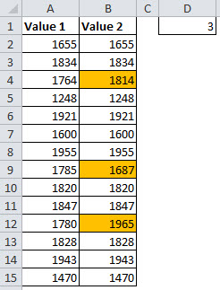
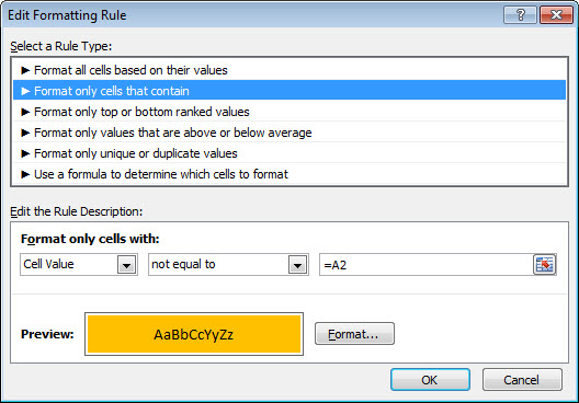
I have used the following Conditional Format on the range B2:B15 to highlight mismatches.

The formula in D1 saves you having to scroll down the whole list to see if there are any mismatches. If there are mismatches, it tells you how many to look for.

The formula in cell D1 is

=SUMPRODUCT((B2:B15<>A2:A15)*1)

Each cell in B2:B15 is compared to the corresponding row in column A. If they are not equal it will return TRUE. The less than and greater than symbols used together <> means not equal to.

In Excel when you multiply by TRUE it is the same as multiplying by 1. If you multiply by FALSE it is the same as multiplying by zero.

So the *1 at the end of the SUMPRODUCT converts all the TRUE and FALSE results into 1’s and 0’s. The SUMPRODUCT function then adds up all the 1’s to, in effect, count the number of entries that do not match.

If you wanted to use the formula in an IF function to display a message you could use

=IF(SUMPRODUCT((B2:B15<>A2:A15)*1)=0,"OK","Error")