When creating ranges of formulas that you want to copy down, you sometimes have a trade off in the use of fixed and relative references. If you need to create a relative reference that acts like a fixed reference you can use a trick.

This technique may not work in all situations, but you might be able to adapt it.

Have a look at the structure below – I am using states as the variable that changes. The more variables you have, the more time this technique will save you.

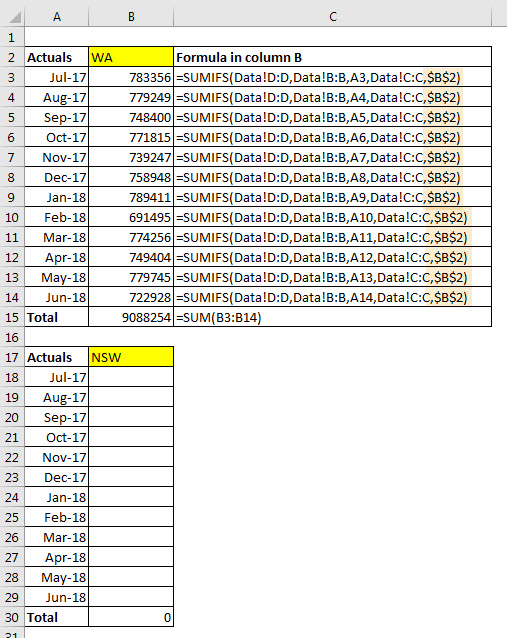
Cell B2 and B17 are inputs

The formula in cell B3 is

=SUMIFS(Data!D:D,Data!B:B,A3,Data!C:C,$B$2)

This formula has been copied to all cells down to cell B14.

I now need to copy the range B3:B14 to B18:B29. The problem is that I have fixed references to cell $B$2 in all the formulas.

I will need to change each one to refer to cell B17 rather than B2 after I paste it to the range below.

The Solution

It only takes a few seconds to adjust the range B3:B14 so that you can copy and paste it as many time as you need into the structures below without requiring any changes.

1. Select the range B3:B14
2. Press Ctrl + H this opens the Find and Replace dialog
3. Type $ in Find box and click Replace All button

That’s it – all the $ signs have been removed.

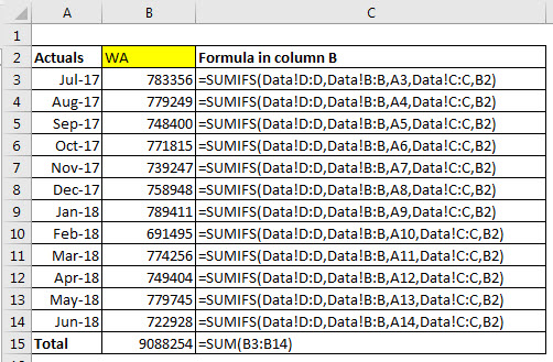
You can now copy the range B3:B14 to B18:B29 and it will work perfectly.

WARNING: This works because the only $ signs in the formula were for the reference we needed to change. If there were other $ signs in the formula then this technique may not work.