It’s finally here, well it is if you have the monthly update cycle of the subscription version of Excel.

This is the new function we have been anticipating for a while now. It simplifies looking up entries from a table and it removes many of the limitations of VLOOKUP. It also adds some features that INDEX-MATCH has, but VLOOKUP doesn’t.

In the image below we can see the XLOOKUP function in action.

In this first article on XLOOKUP let’s see how it let’s you do a look up to the left or above.

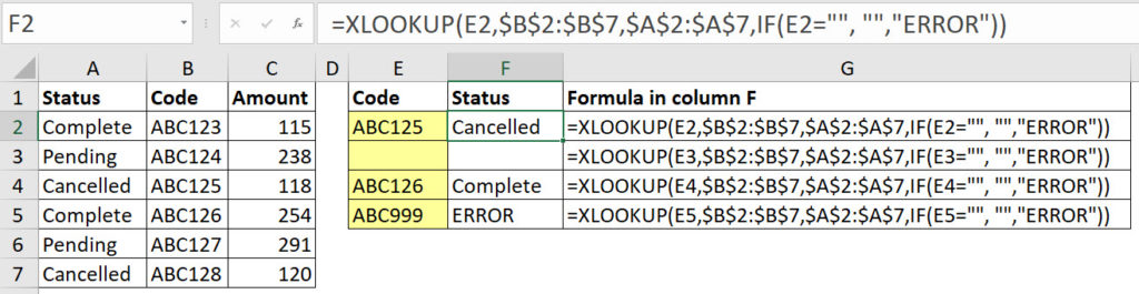
Column G displays the formula for column F.

Syntax

XLOOKUP(lookup_value,lookup_array,return_array,[if_not_found],[match_mode],[search_mode])

lookup_value – the value to lookup, usually a cell reference. The same as VLOOKUP or HLOOKUP.

lookup_array – this is the range to look in. This is not a table reference. It can be a single vertical column or a single horizontal row. Usually a fixed reference.

return_array – this is the range to extract from. Can be a single column or multiple columns. Can be a single row or multiple rows. If multiple columns or rows are defined then the formula will “spill” across as per dynamic array entries.

if_not_found – optional – what to display if the entry is not found. Can be another function like the IF function. Text needs to be enclosed in quotation marks. If omitted the N/A error is returned for entries that can’t be found.

match_mode – optional – the type of match performed. 0 = exact match (default). -1 = exact match or next smallest. 1 exact match or next largest. 2 = wildcard match. Defaults to the exact match if omitted.

search_mode – optional – the type and direction of the search. 1 = search from first (default).  -1 = search from last. 2 = binary search ascending order. -2 = binary search descending order. The ascending and descending options require the lists be sorted accordingly. Defaults to search from first if omitted.

The match_mode argument (5th argument) wildcard option 2 means you can use the *, ? and ~ characters to represent unknown characters.

In the image above I have used the first 4 arguments and accepted the defaults for the last two. In most cases the defaults for the last two arguments are the common requirements.

The formula in cell F2 is

=XLOOKUP(E2,$B$2:$B$7,$A$2:$A$7,IF(E2="", "","ERROR"))

You specify the code to lookup – the entry in cell E2 (ABC125). The range to look in is B2:B7 and the range to extract from is A2:A7.

I have used an IF function in the if_not_found argument.

IF(E2="", "","ERROR")

This displays a blank if cell E2 is blank and the word ERROR if the entry is not found.

This is an easy way to handle blank look up cells and avoid the #N/A error.

Horizontal lookups

Whilst vertical lookups are by far the most common, there can be a need for horizontal lookups and XLOOKUP can handle them too.

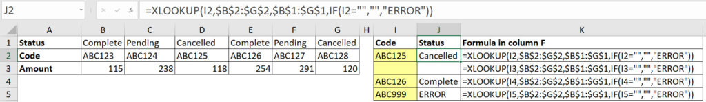
This is the same data but transposed to go across the page. The formula in cell J2 is

=XLOOKUP(I2,$B$2:$G$2,$B$1:$G$1,IF(I2="","","ERROR"))

We can specify a horizontal range to look in, B2:G2 and extract from, B1:G1. The same IF function is used to handle blanks and errors.

I will write more posts on using XLOOKUP in the coming weeks and months.