In a financial model you often have different types of allocations that start at different times. Creating a short formula to handle this flexibility can be a challenge. Here is one solution.

You can download the example file using the button at the bottom of the post.

Below is a table of different types of allocations and number months.

This is in a sheet called Allocation Table.

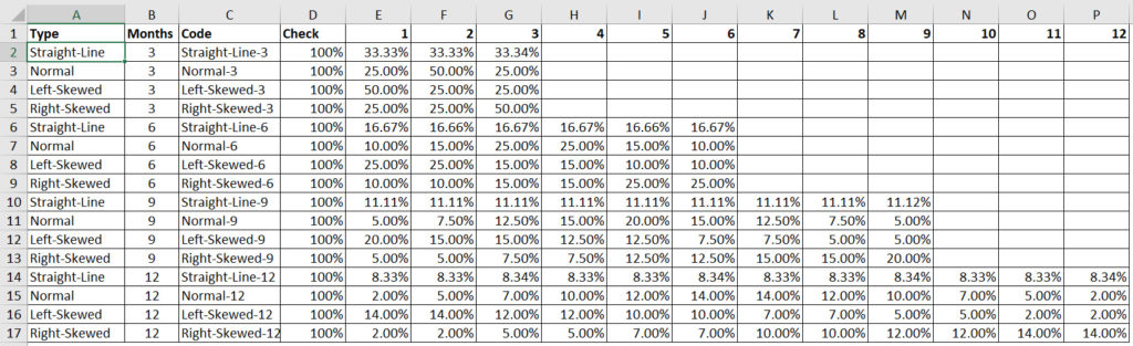
There are four types of allocations.

• Straight-Line – spend is evenly spent across all periods.
• Normal – spend is loosely based on a normal distribution bell curve. Most spend in the middle with the spend building up and tapering off.
• Left-Skewed – most spending occurs early and tapers off.
• Right-Skewed – spending occurs later in the period.

Each type is allocated over 3, 6, 9 or 12 months.

Column C creates a unique code for each row to enable the identification of the allocation.

Column D checks the allocation adds up to 100%.

The cells on the right are all % input cells.

Below is our input and workings section.

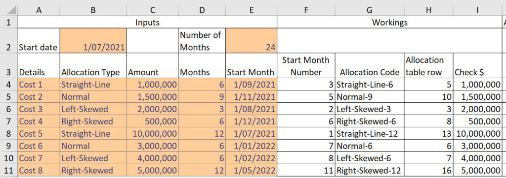
The orange cells are for input.

The range B4:B11 has drop downs to select the type of allocation.

The range D4:D11 has drop downs to select the number of months.

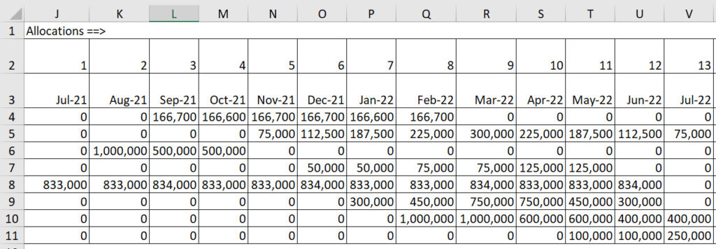
On the right-hand side are the month allocations – see below.

Workings

The working columns make the final formula shorter and easier to create.

The formula in cell F4 is.

=IFERROR(MATCH(E4,$J$3:$AG$3,0),0)

This determines the period number of the start month.

To simplify finding the correct allocation combination I have created a unique code to look up. This combines the type of allocation with the number of months. The formula in cell G4 is.

=B4&"-"&D4

This code matches those in column C of the Allocation Table sheet.

We need to identify the row that this code is in within the Allocation Table sheet. The formula in cell H4 is.

=MATCH(G4,'Allocation Table'!$C$2:$C$17,0)

Column I is a check total to ensure the full amount has been allocated. The formula in cell I4 is.

=SUM(J4:AG4)

These values allow us to create a formula in cell J4 that can be copied down and across to create the correct allocation based on the inputs.

=IF(AND(J$2>=$F4,J$2<=($F4+$D4-1)),$C4*INDEX('Allocation Table'!$E$2:$P$17,$H4,(J$2-$F4+1)),0)

Let’s break this formula down into two parts.

Logical test

The first is the logical test of the IF function. This determines whether an allocation needs to be made.

AND(J$2>=$F4,J$2<=($F4+$D4-1))

The AND function first checks the column period number from row 2 against the start month number from column F. Then it checks the period number from row 2 against the starting period plus the number of months less one.

The less one is needed because the first month is inclusive of the number of months. If period 3 is the start month and you allocate for 6 months you allocate in periods 3,4,5,6,7 and 8. So you finish in period 8 which is 3+6-1.

The AND function checks that the start and end periods fall with the required range.

Allocation

The allocation calculation takes the value from column C and multiplies it by a percentage from the Allocation Table sheet. The INDEX function extracts the percentage from the table.

$C4*INDEX('Allocation Table'!$E$2:$P$17,$H4,(J$2-$F4+1)),0)

$H4 is the table row number from the workings section. It is the row number within the range ‘Allocation Table’!$E$2:$P$17 to extract.

The column number from the table to extract is determined via a calculation based on the column’s period number from row 2.

(J$2-$F4+1)

We take the column period number, subtract the starting period and add one. The first month number to allocate, deducted from the column’s month number will always return zero. Hence, we add 1 because we want the first column from the allocation table. As this part of the formula is copied across it provides a sequential column number to extract from the table range ‘Allocation Table’!$E$2:$P$17.

The end of the IF function returns zero if the period doesn’t require an allocation based on the AND function logical test.

This formula is moderately complex but by using helper cells it’s length is manageable.

It allows a flexible input of allocation plus time frame on a line by line basis.

Download the example file using the button below.

Download Example File