Converting multiple text numbers into real numbers or reversing the sign on multiple numbers is easy in Excel if you know how to use Paste Special.

Many systems don’t output numbers very well to Excel. Either the numbers are text or negatives are shown as positive.

The same technique can fix both of these issues and it doesn’t involve any formulas.

There is a built-in feature that will fix the text number issue – most people don’t know that it exists.

In the figure below cells B2 and B4 are text numbers.

Notice the small green triangle in the top left corner of the cell. That symbol means that there is an error with the cell.

Text numbers are not included in most Excel calculations. Hence it can look like a value is added up but it may not be – that can cause errors. The left alignment of the number is another clue that it is treated as text rather than as a number.

If you select a range that starts with a text number an icon is displayed as per the image below.

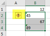
Excel will display a ! symbol (highlighted in yellow above). You can click on this icon to see possible solutions to the error. See image below.

You can fix the error in this case by clicking on the Convert to Number option.

This little icon only appears when the first cell in the range has an error. If you want to adjust the whole column of numbers that may be a mix of numbers and text numbers then you may not see the icon displayed.

To convert a column of numbers when you don’t have the icon present you can use a technique that involves the paste special feature.

Paste Special

Type the number 1 in a blank cell and copy it. Then open up the Paste Special dialog (you can use Ctr + Alt + V). See image below for the two settings (Values and Multiply) required.

The result is shown below when you click OK.

It is a good idea to select the Values option which ensures that the format is not changed. Then you need to select the Multiply option this will multiply all of the cells in the range by 1. This forces Excel to convert any text numbers into real numbers and it won’t affect any real numbers.

Convert to Negative

When trying to convert numbers to negative you can use exactly the same technique. In the image below we want to convert the values highlighted in yellow to negatives.

All you need to do is type -1 in the cell and copy it. Then select the range that you want convert to negative and then open the Paste Special dialog and use Values and Multiply and click OK again.

See images below.

the result is shown below.

This technique enables you to make charges directly to the data without having to enter other formulas and then copy and then paste values and then remove the formulas.