Here is the problem. You have a single column range. Each cell in the range needs to be given a unique range name. Doing this manually takes time, but there is a quick and easy method to do it.

Typically you need to name the cells that are linked to controls such as checkboxes. If you need a series of checkboxes you also need a series of named cells. Entering the names manually is time consuming and prone to error. There is a shortcut technique that can create multiple named cells very quickly.

The companion video below demonstrates how quickly you can apply this technique. It actually takes longer to explain than it does to do it. It takes me less than a minute to create 10 individually named cells.

The image below shows that column E will be used to determine whether or not to apply a surcharge to a product. Eventually a checkbox will be added above each cell in the range E2:E11.

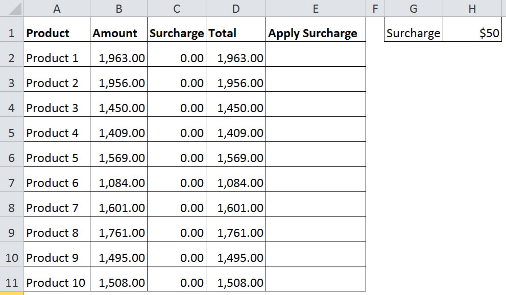
Each cell in E2:E11 needs to be named. The convention we will use includes a prefix. This will be cb for checkbox. It will include the word Surcharge and it will be numbered one to ten. So cell E2 will be named cb_Surcharge01 and cell E11 will be named cb_Surcharge10.

The quick way to do this is to take advantage of two of Excel’s shortcuts. The first is the built-in technique to increment any numbers on the end of text when you use the Fill Handle to drag a cell. And the second is a shortcut to name ranges based on cell labels that are next to the ranges.

We will insert a blank, temporary column between columns D and E. This will contain the range names we want to create.

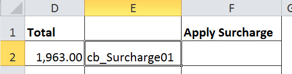
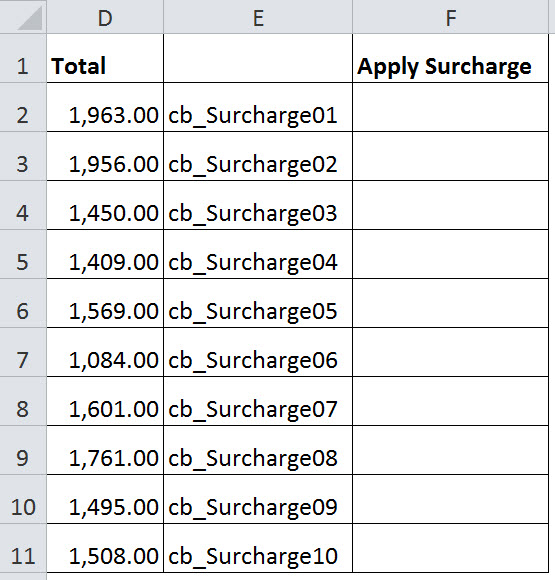
In the new cell E2 we type the first name. We can then double-click the Fill Handle (small black cross bottom right corner of cell) to create the other sequential range names.

We can now select the range E2:F11 and press Ctrl + F3 to open the Create from Selection dialog. This dialog allows you to use the labels in other cells to name cells that are next to, or underneath, the labels.

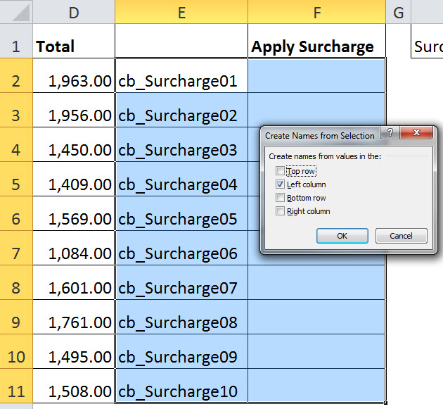
Ensure that the Left column option is the only one ticked and click OK. This will create ten new range names based on the entries in column E.

That’s it, done!

You can now delete column E which we only needed temporarily and the sheet is now ready to add the checkboxes which can then be linked to the named cells underneath.

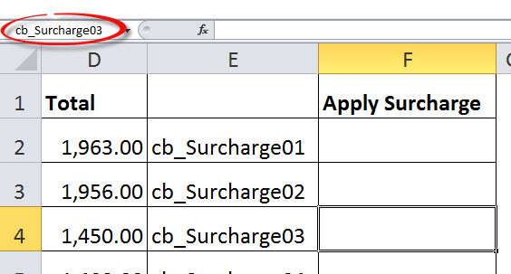
Clicking a cell will show you the name in the Name Box – see image below.