A client recently had a problem. He was chasing a formula that identified if a text string contained one of three words. He wanted to base an allocation on finding those three words. SUMIFS offers a solution.

To demonstrate the problem and the solution I have recreated the structure in the image below.

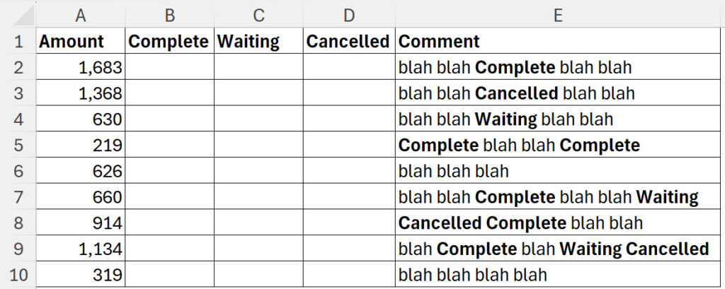
Based on the Comments in column E, the amount from column A needs to be allocated to either column B, C or D based on the column name in row 1.

As an example, row 2 needs to be allocated to the Complete column (column B). Row 4 needs to be allocated to column C, the Waiting column.

Now you might think you should use the SEARCH function. But the problem with the SEARCH function is that it returns an error if it can’t find what it’s looking for. That means you must handle errors. Typically you have to use another function with SEARCH like ISNUMBER. Why use two functions when you can use one.

SUMIFS Solution

SUMIFS can use wildcards like the * symbol to represent any character.

SUMIFS adds up values based on a condition. That condition can contain the * symbol. Typically, SUMIFS is used with a range, but you can also use it with a single cell.

The solution formula for cell B2 which can be copied across and down is.

=SUMIFS($A2,$E2,”*”&B$1&”*”)

The formula has been entered in cell B2 and copied across and down in the image below.

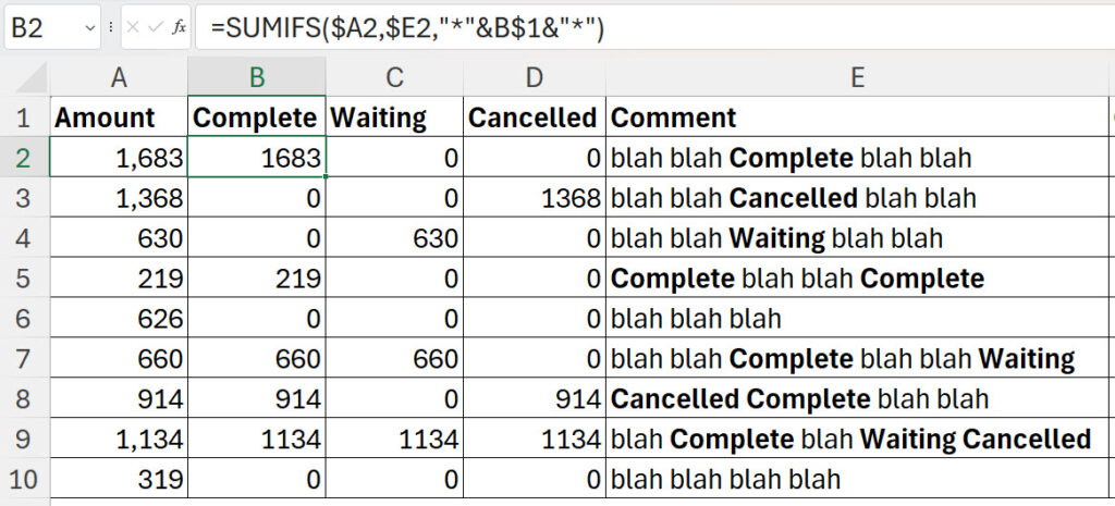
The SUMIFS function looks in cell E2 and tries to find the entry in cell B1. By surrounding the entry from B1 with  the * symbol it will find if that word appears in the cell.

If the word is found in column E the value in column A is returned.

One of the issues we face is that more than one of the words could appear in column E. See row 7 as an example.

We need a way to identify if a row needs to be manually checked.

A simple SUM will handle this problem.

In column F we can create a formula that will return TRUE if the row needs to be manually reviewed. The formula for cell F2 is.

=SUM(B2:D2)<>A2

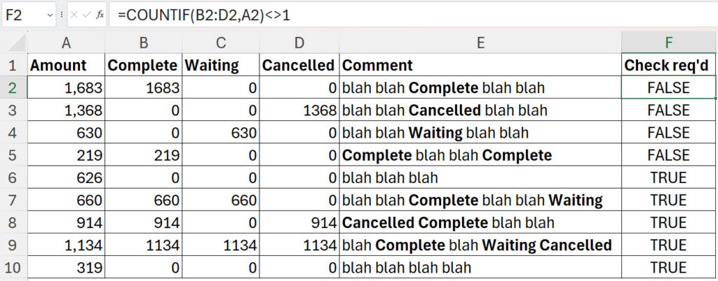
If the three columns add up to column A then FALSE is returned. If they don’t TRUE is returned. TRUE is returned when the word is not found in column C. TRUE is also returned if more than one word appears. Multiple instance of the same word is OK – see row 5.