With the introduction of Dynamic Arrays in all versions of Microsoft 365 (formerly Office 365) it is now a lot easier to use the TRANSPOSE function.

The TRANSPOSE function links to the source range and switches rows to columns and column to rows.

In the old version of Excel you had to

• know how large the output range was and select it and
• use the Ctrl + Shift + Enter (array entry)

This made using the function cumbersome. Now it is easy. Those two requirements have been removed.

Reminder – currently this only works in the subscription version of Excel.

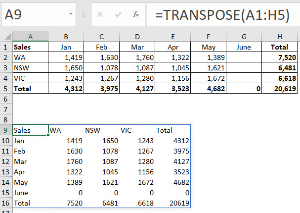
We need to switch the report below so that the months go down the sheet.

That is now as easy as entering the following formula in cell A9.

=TRANSPOSE(A1:H5)

That’s it.

You can see the result in the image below.

The blue line around A9:E16 is called the Spill range. The formula is entered in cell A9 and “spills” to the rest of the range. Excel “knows” how far to extend based on the range used. There are no formulas in the other cells in the range. The only formula is in cell A9.

This creates links back to the original cells.

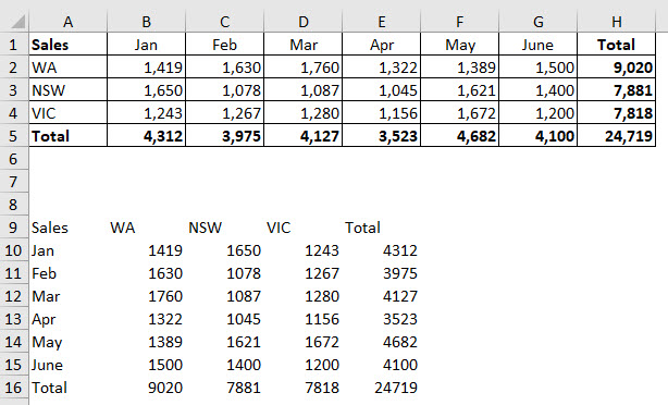
If I enter values in June it automatically updates – see image below.

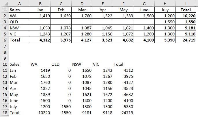
Inserted rows and columns

If I insert rows and/or column it is handled seamlessly – see image below.

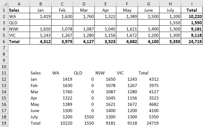
Moving a spilled range is easy.

Simply move the top left cell of the range and the spill range moves with it.

I dragged cell A10 to B11 – see image below.