I wrote a blog post a while back about outliers and Excel and I thought I would revisit it thanks to dynamic arrays.

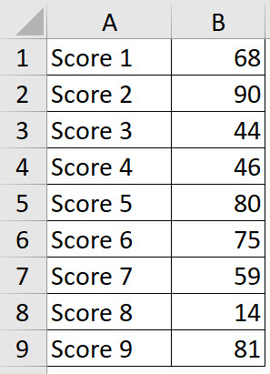
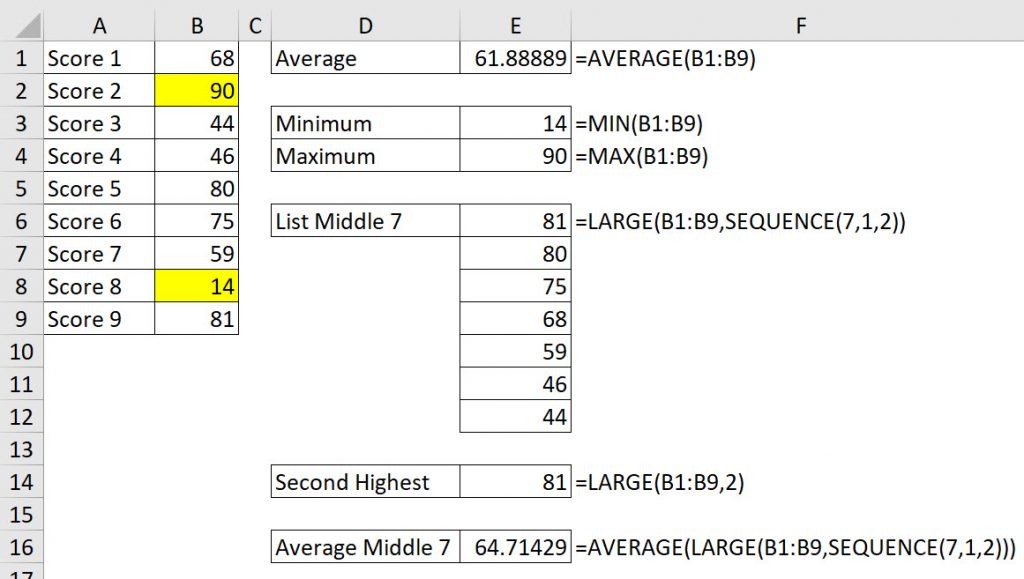
Let’s say we have 9 scores as below.

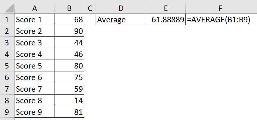
We need to calculate the average of the scores. That is easy with the AVERAGE function.

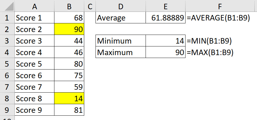
Now, let’s say we wanted to treat this like the Olympics and remove the highest and the lowest scores (yellow cells) and get the average of the remaining scores.

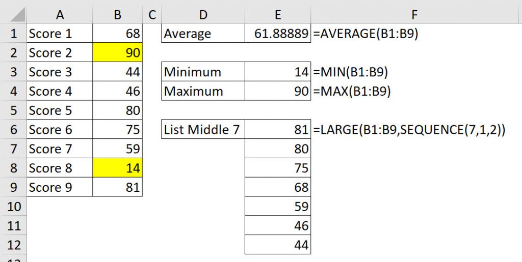
We can use the LARGE function and the SEQUENCE function together to create a list that excludes the highest and lowest scores.

The LARGE function is like the MAX function except it allows you to extract values based on position. So it can extract the highest (1) or the second highest (2) all the way down the lowest value.

In our case the following formula would return 81 – the second highest value.

=LARGE(B1:B9,2)

To create a list of the scores we need, we have used the SEQUENCE function as the second argument in the LARGE function.

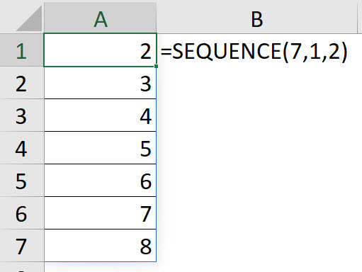
=SEQUENCE(7,1,2)

The creates a list of sequential numbers as shown below.

This list ignores the first (1) and last (9) numbers and give us the numbers from 2 and 8.

To work out the average of the revised list (the middle 7) we can use the LARGE and SEQUENCE function formula as the range for an AVERAGE function.

The average result for the middle 7 scores is slightly higher that the average for all the scores.

Let’s say we want to be more conservative and exclude the top two and bottom two scores. What formula would we use?

Leave suggestions in the comments below.