Formatted Tables are great but there is an issue when it comes to copying formula that use the table names (Structured References). There are two techniques that cope with this limitation.

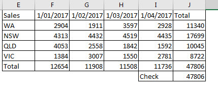
Have a look at the image below. The data on the left is summarised in the report on the right. (Yes, we could use a PivotTable, but this is a formula demonstration).

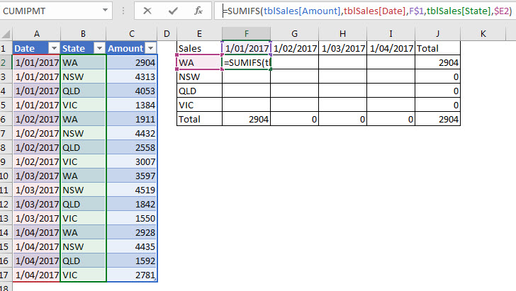
The formula in cell F2 is shown in the Formula Bar.

=SUMIFS(tblSales[Amount],tblSales[Date],F$1,tblSales[State],$E2)

The references you see in the SUMIFS function are called Structured References.

tblSales[Amount]

The one above refers to the Amount column in the Formatted table named tblSales.

Formatted Tables are always named. Excel provides a generic name like Table1 when you first create a Formatted Table. You can change the name to be more descriptive. When the table is selected a Design ribbon tab appears and the name box is on the far left-hand side. I use a prefix of tbl for my Formatted Tables.

See my previous posts below on Formatted Tables if they are new to you.

https://a4accounting.com.au/format-as-table-in-excel-part-1/

https://a4accounting.com.au/excel-format-as-table-part-2-video/

Let’s be honest the term Structured Reference doesn’t describe what they are. They are table names – names that relate to a Formatted Table. I call prefer to call them table names to be more descriptive.

The SUMIFS function performs single or multiple criteria SUM calculations. It was introduced in Excel 2007. In the formula above the SUMIFS function is adding up all the values in the Amount column when the State column equals WA (cell E2) and the when the Date column equals 1/1/17 (cell F1).

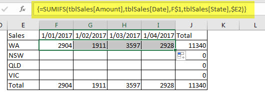
Because we have used the $ signs around the cell references in the formula you would expect we could use the Fill Handle (small black cross bottom right corner of cell) to drag the formula across to copy it. But we would be wrong – see image below.

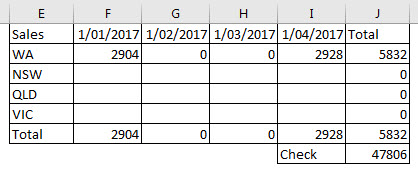
The problem is that when you use the Fill Handle to copy the table names across, the table names change just like relative cell references. When we look at the formula in cell G2 after we drag we can see the effect.

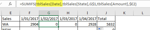
The reference to the Amount column at the start of the SUMIFS has changed to the Date column – what has happened?

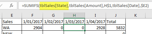
As I mentioned the table names change as you drag them across. Because the Amount column is on the far right of the table it reverts to the first column in the table, the Date column. The SUMIFS in cell H2 starts with the State column

By the way you can always use the Fill Handle to copy the formula down a column as this doesn’t affect the column references. Its copying across columns that has issues.

Solution 1 – Simple

The easiest solution it to simply copy and paste the formula. This is what I recommend in all my training sessions. When you copy and paste the formula the table names don’t change and you get the result you expect.

Solution 2 – Advanced

This is more advanced and it allows you to use the Fill Handle to copy the formula across. When you enter the formula in cell F2 you can use Ctrl + Shift + Enter (array entry) to enter the formula. This places the curly brackets (braces) around the formula. You can then use the Fill Handle to copy across. The array entry stops the table names from changing as you copy it across with the Fill Handle.

My preference is to use Solution 1, but if you already use arrays you may prefer Solution 2.