Some systems add DR and CR to the end of numbers when they export into Excel. This renders the values useless for normal calculations. You can use data cleansing techniques to remove the characters using formulas or Power Query. There is one function however that can perform calculations on these types of entries.

SUMPRODUCT can perform calculations on text-based numbers which I covered in a previous post. It can even calculate when there is text in the numbers. Take a look at the screenshot below.

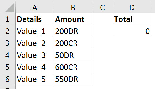
Most functions can’t perform numeric calculations with the entries in column B, but SUMPRODUCT can.

We want to ensure that these values balance, they may be from a journal entry. It can be tricky performing this calculation because if you get the calculation wrong it may display zero anyway. It is always a good idea to test by changing one of the values so that it doesn’t balance to make sure that your formula is working correctly (see end of post).

The formula in cell D2 is

=SUMPRODUCT((LEFT(B2:B6,LEN(B2:B6)-2))*((RIGHT(B2:B6,2)="DR")-(RIGHT(B2:B6,2)="CR")))

This type of calculation is impossible with most of Excel functions but SUMPRODUCT can work with ranges of data. This also demonstrates how to use a mutually exclusive logic calculation within the SUMPRODUCT brackets. The mutually exclusive technique is discussed below.

The way we want to handle these entries is that debit (DR) values are treated as positive and credit (CR) values are treated as negative. All of the entries have either DR or CR.

(LEFT(B2:B6,LEN(B2:B6)-2))

The first part of the SUMPRODUCT simply extracts the value from the range in column B. It uses the LEN function to determine how long the text string is and it subtracts 2 to remove the last two digits from the entry. This leaves just the text value.

As mentioned we can’t just use the text value because some values are to be treated as positive and some as negative.

Mutually Exclusive

((RIGHT(B2:B6,2)="DR")-(RIGHT(B2:B6,2)="CR"))

This part of the SUMPRODUCT is the mutually exclusive calculation. It uses an extra set of brackets to enclose and combine the two logic calculations. This calculation can either use the plus sign or the minus sign between the two logic calculations. It depends on what you’re trying to achieve. In our case we are using the minus sign because we are working with either a positive or a negative value.

The first logic test returns TRUE if the last two characters are DR. In Excel TRUE equals one which will convert the text numbers to positives. The second part will return TRUE if the last two digits are CR. Because the minus sign is used between the two logic tests the TRUE for CR will be converted to negative. The net result will either return a 1 or a -1 based on whether an entry has DR or CR. This works because all entries end in either DR or CR.

F9 Technique

When demonstrating these SUMPRODUCT techniques I always use the F9 key to demonstrate how SUMPRODUCT calculates the individual values. The image below shows selecting a certain section of the formula and pressing the F9 function key. This calculates just that part of the formula so you can see how Excel builds up the SUMPRODUCT calculation.

WARNING: the part you select must be able to be independently calculated – missing a bracket can stop the technique from working.

SECOND WARNING: Always press the Esc key after using this technique otherwise the values remain in the formula. You can use Undo if you forget.

The numbered steps are explained below the image

1 & 2 show the conversion of the entries in column B into text numbers by removing DR and CR. The quotation marks ” ” surrounding the numbers mean they are text numbers.

3 & 4 show the identification of DR. TRUE means the entry ended in DR.

5 & 6 show the identification of CR. TRUE means the entry ended in CR.

7 & 8 shows the mutually exclusive calculation which results in either a 1 or  -1 being returned. 1 for DR and -1 for CR.

9 & 10 show the final result that SUMPRODUCT adds up. Either positive or negative numbers. Multiplying the text numbers from steps 1 & 2 by a number converts them into real numbers.

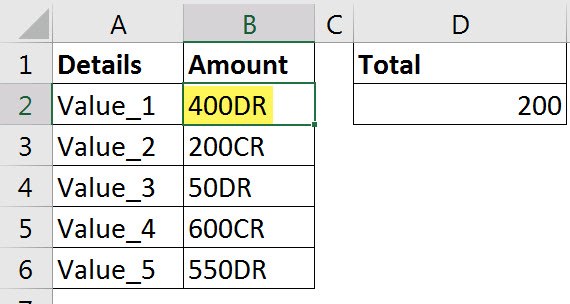
I tested the formula by changing the value in cell B2 from 200DR to 400DR – see result below.