Do you use the “Filter by Selected Cell’s Value” option? If you do then you will be pleased to know there is a Quick Access Toolbar icon that applies it in one click.

WARNING: This tip doesn’t work in a formatted table.

If you are unsure about the Quick Access Toolbar check out this blog post below.

Customizing Excel 2007 and 2010 [VIDEO]

Shout out to Mr Excel (BIll Jellen) as I found this tip in one of his books.

Back in the old days AutoFilter was the name Excel used for the filtering drop downs. In more recent versions that name was changed to Filter.

Also back in the old days there was an icon that was incorrectly labelled and it is the one that now provides the “Filter by selected cell’s value” option.

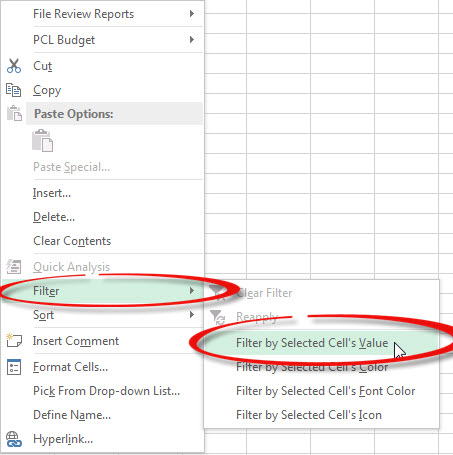
That option is usually accessed via the right click menu, but that takes three clicks to use – see image below.

To add the icon to the Quick Access Toolbar, right click the Quick Access Toolbar (it is either above or below the ribbon and already has small icons on it).

Choose Customize Quick Access Toolbar.

From the Choose commands from drop down select All Commands.

Scroll down the list beneath until you find AutoFilter and select it.

Click the Add button and you are done! See image below.

You can now click an entry in a table and click that new AutoFilter icon to filter by that cell’s value. The icon should appear on the end of your Quick Access Toolbar.

It automatically adds the filtering drop downs to the table if it wasn’t already turned on.