In a previous blog post I explained how to do a 3D SUM calculation in Excel that SUMs through sheets. You can view it here. I have seen a few posts in forums recently about performing a 3D SUMIF calculation. Whilst the SUM function can work with 3D ranges, the SUMIF function can’t.

These solutions relied on the INDIRECT function. Below is an alternative that doesn’t use INDIRECT and hence handles the cases where the sheet names change, which can be a limitation of the INDIRECT technique.

I will use the CHOOSE function which is powerful for two reasons. The first is it has the ability to return ranges. The second is it can use the array syntax in its Index_Number argument (see syntax below). These two features allow us to create a reasonably straight forward solution for a 3D SUMIF using CHOOSE with SUMPRODUCT. A link to the example file is at the bottom of the post.

The syntax of the CHOOSE function is

CHOOSE(Index_Number, Value_1,Value_2, …)

The Index_Number selects a value from the list of values on the right. Each Value (Value_1, Value_2, etc) can be text, a number, a cell or a range.

Example

=CHOOSE(2,A1,B1,C1)

will return whatever is in cell B1 because it is the second (2) value listed.

We can use the array syntax {1,2,3} within the Index_Number argument to select multiple ranges one after the other.

Worked Example

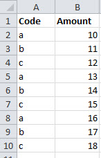
We have three separate Data sheets named Data1, Date2 and Data3, with codes in column A and amounts in column B, see image below.

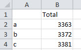
The Report sheet (see below) summaries the threes codes a, b and c from all three sheets.

The formula in cell B2 in the Report sheet is:

=SUMPRODUCT((CHOOSE({1,2,3},Data1!$A$2:$A$10,Data2!$A$2:$A$10,Data3!$A$2:$A$10)=A2)*
 (CHOOSE({1,2,3},Data1!$B$2:$B$10,Data2!$B$2:$B$10,Data3!$B$2:$B$10)))

The first CHOOSE function defines the three ranges that have the codes. The {1,2,3} at the start of the CHOOSE will select each of the three ranges one after the other and then compare them to the value in A2. This will return a series of TRUE and FALSE results based on whether the cell in the range matches the value in A2.

The second CHOOSE function returns the three separate amount columns one after the other using the same array syntax technique. These align perfectly with the Code columns and the values in those columns are multiplied by the TRUE and FALSE results.

In Excel TRUE =1 and FALSE = 0.

Hence, all the values that didn’t match A2 will return FALSE (zero) and be multiplied by their corresponding value and return a zero. When the values are multiplied by TRUE (one) they return their respective value. All these “correct” values are all added up by the SUMPRODUCT function to return the SUMIF result.

You can replace the ranges used in the CHOOSE function with range names, which can shorten the formulas.

Example file 3D_SUMIF