Data Validation and Conditional Formats in Excel

In my previous post I showed how to have a flexible data validation and how to validate it. This post will look at adding conditional formats to inputs and validations.

You can see the previous post here.

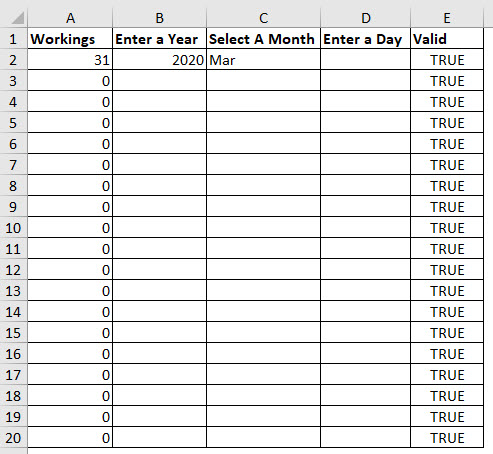
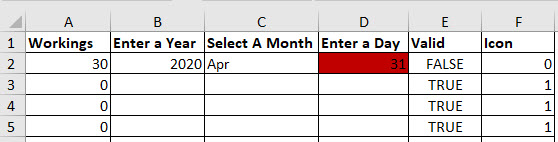
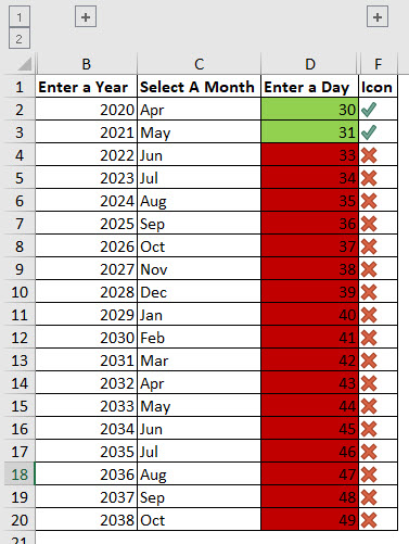
This image below is where we left off in the last post.

You can download the example file via the button at the bottom of the post.

We are not worried about formatting the year and month entry.

We can use a conditional format on the day entry column to highlight when it is invalid.

Because we have used a logic calculation in column E to validate column D this process is straight forward. Conditional formats use logic calculations to identify when to apply formats.

Colour blindness

When working with conditional formats the typical red/green colour combination works for most people but there is a small percentage of people, mainly men, who have some form of colour-blindness. Red green colour-blindness is the most common. We will use the red/green combination but also add a tick/cross icon that will help those who are colour-blind.

Applying the conditional formats

Select the range D2:D20.
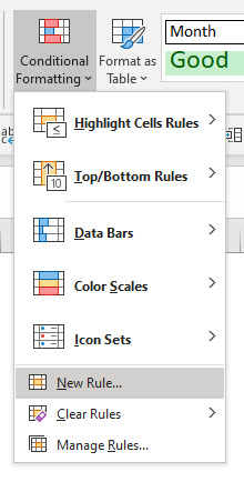
On the Home ribbon click the Conditional Formatting icon drop down and select New Rule.
Select the last option in the top section “Use a formula to determine which cells to format”
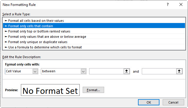
In the Formula box enter the following formula
```
=$E2
```
When creating a formula for a range it is important to build the formula to work with the first cell in the range, in this case cell D2.

The formula you create must return TRUE to apply the format. Since we already have a cell with TRUE/FALSE we can just refer to it.

It is also important to use the $ signs correctly within the formula. In the example above we need the row number to change for the rest of the range hence it doesn’t have $ sign in front of it. The column doesn’t change, so we used the $ sign in front of the column reference.

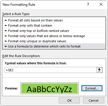
Click the Format button and on the Fill tab add a green fill colour and click OK. The dialog should look like the image above. Click OK.
This will highlight all the cells green because we defaulted column D to TRUE if the cell was blank. We will remove the green for a blank option in a later step.
With the range still selected create another New Rule. It is also a formula-based rule.
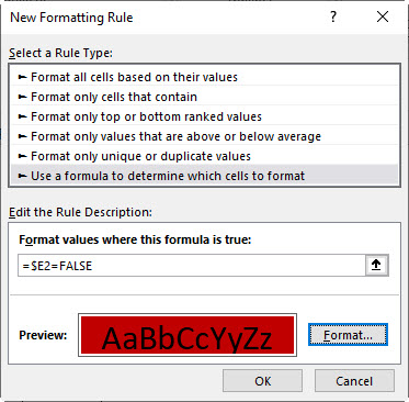
The formula to be entered is
```
=$E2=FALSE
```
Remember the formula needs to return TRUE to apply a format. In this case we need to identify an invalid entry, so we compare the cell to FALSE.
Click the Format button, on the Fill tab select a red colour and click OK. The dialog should look like the image below. Click OK.
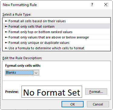
We need to add another condition a blank cell. This won’t apply any formats. With the range still selected create another New Rule.
This time select the second option – “Format only cells that contain”
In the bottom section in the left hand drop down select Blanks and click OK. We don’t need to set a format.
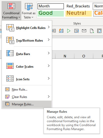
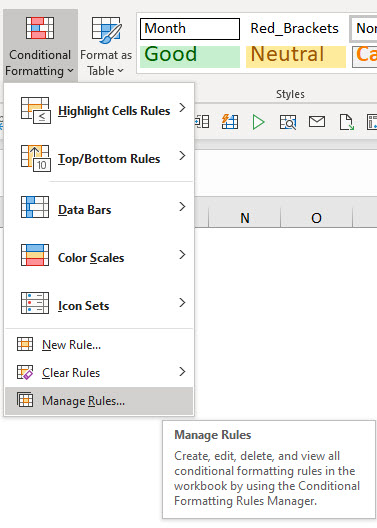
We have created three separate conditional formats. We need to change as setting to make them work correctly. Click the Conditional Formatting icon and select the last option, Manage Rules.
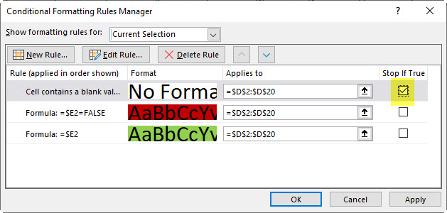
In the image below the three conditions are listed (image below), but we need to ignore the last two conditions if the first condition is met. We can use the “Stop if True” check box option on the left of the first rule to do that. When you tick that box the conditions below will not be used if the condition is met. Click OK.
The green cells will disappear for the blank cells.
Try a few entries to break the validation, eg change the month after the day to create an invalid combination like 31 April.
Adding a tick or cross icon requires adding another column. The icon set in conditional formatting requires numeric entries and won’t work with TRUE/FALSE entries. Luckily it is very easy to convert TRUE and FALSE to a numeric. Insert a new column to the right of column E.
The formula to convert TRUE/FALSE to numbers in cell F2 is
```
=E2*1
```
You could also use
```
=E2+0
```
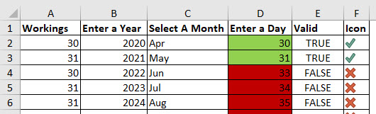
This technique is called coercing the value. By performing a calculation with a logic result you force (coerce) Excel into converting TRUE into 1 and FALSE into 0 – their binary values. So TRUE will display 0 and FALSE will display 0. See image below.
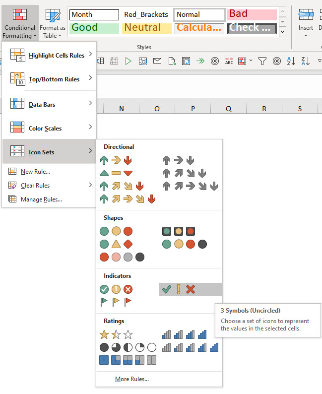
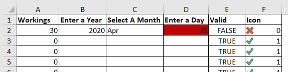
To add the icons we select the range F2:F20 and click the Conditional Formatting drop down and select Icon Sets. I prefer the Tick and Crosses in the Indicators section as per the image below.
This applies the default settings which appear to work, but they do have a problem.
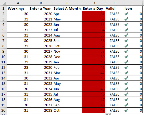
If all the entries are FALSE if will display ticks – see the image below where I have copied down row 2.
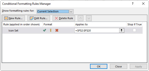
The icon set default settings aren’t always best, so you need to amend them. Select the range F2:F20 and click the Conditional Formatting drop down and chose the last option Manage Rules.
In the dialog that opens double click the Icon Set line.
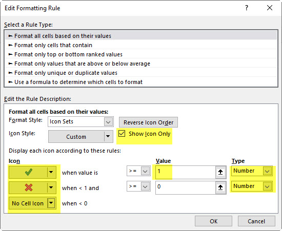
I have highlighted in yellow the changes you need to make in the Edit Formatting Rule dialog below.
Click OK and OK again. Problem solved.