Power Query Zoom
I used this today in a live webinar.
I zoomed into the Power Query window in Excel to make it easier to see.
Ctrl + Shift + + (plus)

I used this today in a live webinar.
I zoomed into the Power Query window in Excel to make it easier to see.
Ctrl + Shift + + (plus)
20 years ago I had an article published on Excel shortcuts keys – let’s revisit it.
When you are working with text numbers in tables sometimes you need to convert real numbers into text numbers to do look ups.
There are at least two ways to do this.
Let’s see how to convert real numbers into test numbers, real fast.
In Australia our financial year starts in July. Excel is set up to work with calendar years and we need to do some date gymnastics to have our reports start in July. Here is a hack for Custom Lists that can make some things better in Excel.
When you import numbers from other systems they sometimes come in as text and are left aligned.
There are a couple of ways to fix them and they can both be done in less than a minute.
You need the Developer ribbon tab visible to record a macro, or do you?
This old-fashioned keyboard shortcut will open the record macro dialog. Pressed in sequence, not held down.
Alt T M R

You can also use the little icon next to the Ready at the bottom left corner of the screen.

Once you start recording the small square icon to stop recording appears in the same spot.

My first article was published on 10 August 2001 in the Accountants Weekly magazine.
I have scanned the original article and it is shown below.
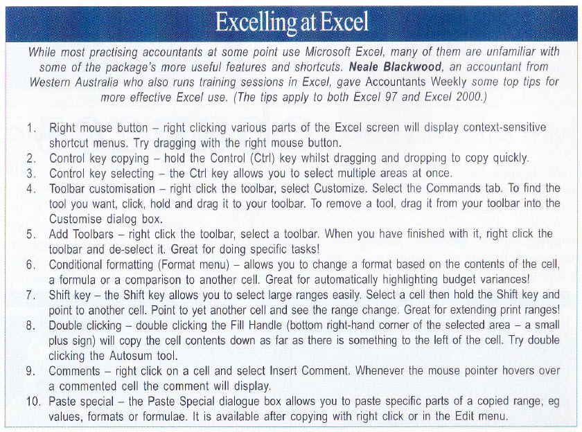
20 years later I thought I would update the 10 points from the article.
When published all those years ago these tips applied to both Excel 97 and Excel 2000. We have come a long way since those days.
The Merge cells format has lots of issues. It can crash macros and stop you copying and pasting.
In less than a minute you can use a macro to solve the problem.
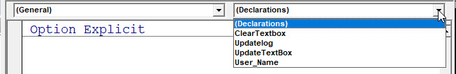
Did you know the right-hand side drop-down, above the code window, lists all the Subs and Functions in a module? Now you do.
Replacing colours manually can be a tedious task.
Did you know you can use Excel’s built-in Find & Replace to do the job for you?
Joining names; extracting codes or converting dates is usually done with formulas, but there is now a formula-free solution called Flash Fill.
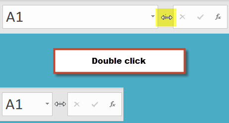
Just found out you can double click the re-size control on the Name Box. This quickly shrinks the Name Box width.
I have no idea how long that feature has been there, but I have just found it. Woohoo!
When you have a filter in place in Excel you typically only affect the visible cells when you edit multiple cells. There is a case when you are affecting all cells not just the visible ones.
A check box is an easy interface to create and use.
See how to add one to a sheet and use it in a calculation.
If you need to paste values and formats then you can use a single keyboard shortcut after you have copied.
Alt H V E will paste both.

You can’t hide a cell, but you can stop the cell value from displaying on the sheet.
It involves a custom number format.
If you have cell selected in the output table from a Power Query, you can press, in sequence (not held down) the following keys Alt P U E to open the Power Query Editor window.

Often people perform calculations off to the right of Pivot Tables to calculate percentages.
In this short video I show you those calculations can be done inside the Pivot Table itself.
The solution is not intuitive, but it is easy.
This example builds upon the previous One Minute to Excel post.
If you need to extract the Australian Financial Year from a date in Power Query here is how to do it.
I typically use the shortcut Alt A V V pressed in sequence (not held down) to open the Data Validation dialog.
I like it because you can do it one-handed. The A and V are close together.
There is another shortcut that works the same. Again, pressed in sequence and not held down. Alt D L

Use the one that is easiest for you.
Here’s a couple of useful keyboard shortcuts for Pivot Tables.
Display/Hide the Pivot Table Field List – this list lets you create or change the Pivot Table.
Alt J T L – pressed in sequence, not held down.

To add Subtotals above the entries in an existing Pivot Table.
Alt J Y T T – again pressed in sequence, not held down.

Note sure why, but Pivot Tables are often seen a “hard” or “advanced”.
In the short video we see how easy they are.
Oops – I go over my one minute time limit by a few seconds because I format the Pivot Table as well.
The Formula Bar can be expanded using the icon on the end. But there is a keyboard shortcut as well.
You can expand it or return it to one line using the keyboard shortcut Ctrl + Shift + U.
Thanks to Excel MVP Tom Urtis for sharing this shortcut recently on LinkedIn.

This short video covers different ways to insert a drop down list into a cell.
I go over my one minute time limit by a couple of seconds, but I do cover three techniques.
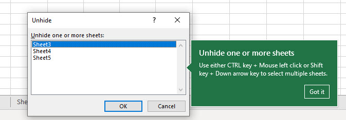
Well, the wait is finally over in the subscription version.
You can now unhide more than one sheet at a time – woohoo!
When you paste into Excel from other applications, sometimes the formats can be problematic. Here is a tip to ignore formats.
Yes, you can create a cell drop down without Data Validation. It uses a built-in technique and is flexible.
Copying is a common task in Excel. This technique applies to most things in Excel form cells and range to charts, images and sheets.
It also works in Word and PowerPoint.
Have you used the mouse and keyboard together? It is time to start.
Let’s go.
When you protect a sheet in Excel many icons are turned off (greyed out), including the ever popular AutoSum icon. That’s when it pays to know keyboard shortcuts.
This link above is a great resource for Power Query data connectors.
It is listed alphabetic order.