If you have a list of numbers that are a text numbers or a combination of text numbers with real numbers there is a technique I covered in this blog post to add them up. But if the range also contains text then the technique won’t work. There is the work around. The solutions below work in the subscription version of Excel. Check the comments section below for a solution for all versions.
Category Archives: Functions
The Magical N Function in Excel
Who you calling short?
One reason I like the N function is because it is Excel’s shortest function name. But it has quite a few useful features as well.
Last used column number in a row in Excel
AGGREGATE to the rescue
A while back I posted a formula to find the row number of the last used cell in a column. I revisit the solution to provide the last used column number in a row.
Removing Outliers in Excel
Dynamic array solution
I wrote a blog post a while back about outliers and Excel and I thought I would revisit it thanks to dynamic arrays.
The Excel CONVERT function
Most conversions are easily done
If you need to convert between different measurement systems Excel has just the function for you, called CONVERT.
Working with a Different Working Week in Excel
International functions to the rescue
Let’s say you are transitioning to retirement (lucky you) and you only work four days a week. You have Wednesdays off to play golf. You may still do projects and you need to figure out completion dates based on a start date and working days. Excel can help you.
Switching Reports from Rows to Columns in Excel
TRANSPOSE and OFFSET solution
I was recently helping someone with a budget which they had built vertically, with the months going down the sheet. They then asked to display it horizontally, with the months going across the page. In the latest version of Excel this is straightforward.
Dynamic Arrays and a Book Index
Another solution
Years back when I wrote my Excel book, I had to create an index for the book. I shared the file I used including the macro in this post. Recently I thought dynamic arrays could do much of the work for this.
Financial Year Month in a Pivot Table
Create new column
I wrote an article years ago explaining how to use a related table to handle financial years in Excel Pivot Tables. You can read the article here. If you only want the months in financial year order you can just add an extra column to your table.
Extracting Time from Date and Time in Excel
Another MOD function solution
I had a recent query regarding checking time in a column that had both date and time. There is an easy way to extract time from a date-time combination.
Conditional Format to Display Only the First Entry
In my previous blog post I showed a technique to reduce clutter. The technique used a manual formatting method. Here is the automated version.
You can see my previous post here.
Below is the original table.
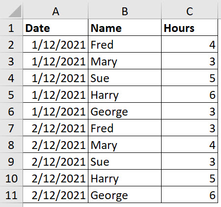
We can use a Conditional Format to only display the first entry of each date in the Date column.
Select the range A2:A11.
Click the Conditional Formatting drop down and select New Rule (third from the bottom).
Select the last option in the top section “Use a formula to …”.
In the formula box enter the following formula.
=COUNTIF($A$2:A2,A2)>1

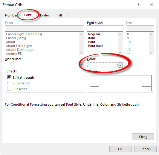
Click the Format button and use the Font tab and change the font colour to White and click OK and then OK again.
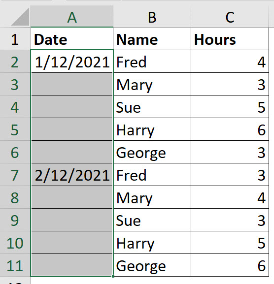
The result is shown below.
The formula for a conditional format must return TRUE to trigger the format. The type of formula that you use is called a logical test, which returns either TRUE or FALSE.
The use of the $ signs is very important in this formula. The COUNTIF function counts the number of entries in a range. If the COUNTIF result is above 1 it is a duplicate. In cell A2 the formula will ALWAYS return 1 as it is counting itself.
When creating a formula-based condition across a range you need to build the formula to refer to the top left cell of the range. In this case we need the range to expand as the range extends down the sheet. Hence, we didn’t use any $ signs on the last two A2 references used.
In cell A3 the formula will be.
=COUNTIF($A$2:A3,A3)>1
This is because the A2 references in the original formula had no $ signs, so they will change with the cell to A3. In our case this COUNTIF will return 2 because the date in cell A3 is a duplicate of the date in A2. This will trigger the format.
This formula expands as the range extends. It uses the cell reference of the cell it is in to determine if the entry is the first entry or a duplicate. This formula will not change the format of the first entry, but it will change the formats of any duplicates.
Let’s TRIM with Dynamic Arrays in Excel
Removing problematic spaces with a single function
Dynamic arrays allow you to use a function normally built to handle a cell, with a range of cells. The TRIM function can remove extra space characters in cells. So with dynamic arrays it can handle ranges.
Convert text time to real time in Excel
Three different ways
I recently downloaded an example file for an Excel challenge. The challenge had a lot of things to do but they were all based on a Timestamp column that had text instead of times.
Find the Closest Value in Excel
Dynamic array solution
On LinkedIn recently someone posted an Excel formula solution lamenting that it was long and complex. That of course was a challenge to me to simplify it.
Time differences in Excel
ABS to the rescue again
Here’s a technique to calculate the time differences when you aren’t sure which time is first or last. Note with standard Excel settings you cannot report negative time.
Back when text was just text
Text functions revisited
20 years ago my last article for the Accountants Weekly magazine was published. They spelled my name wrong after getting it right for all the other articles, maybe that’s why I stopped.
Twenty Years Ago – Top 10 Excel Functions
How things change
My second article in Accountants Weekly was published 20 years ago today and it was Top 10 Functions for Accountants.
Adding Time in Excel
There's a function for that
If you need to add time to an existing time then you need to learn about the TIME function.
Confirming Names are Unique in Excel
COUNTIFS to the rescue
If you have a list of first names and last names and you want to make sure the list has no duplicates you can use a formula to confirm the names are unique.
Make Sure All Input Cells Have an Entry in Excel
COUNTIF to the rescue
When creating an input range you may need to validate input cells. That may mean ensuring all input cells have an entry. Here’s how.
How Many Rows and Columns in a Range
Two functions to the recue
Excel has two functions to answer these questions.
Distinct Count Formula in Excel
New and old functions combined
It is now easier to create a distinct count formula in the subscription version of Excel. You can also use a criteria. A distinct count only counts each value once. Duplicate entries are ignored.
Australian Financial Year Quarter Formula
Another CHOOSE solution
The Australian Financial Year has its challenges. Working out the Quarter number based on a date has a few solutions. Here’s another one.
Financial Model Allocation Technique
Helper cells to the rescue
In a financial model you often have different types of allocations that start at different times. Creating a short formula to handle this flexibility can be a challenge. Here is one solution.
Handling Formula-Based Blanks
The N function to the rescue
It is common to display a blank cell using the IF function and “”. A problem can arise when you want to use that IF formula in a calculation. Here is an easy way to cope.
Single formula for a Column
It can done
In Excel your goal should be to have a single formula in a table column that can be copied down the whole column.
XLOOKUP Doesn’t Always Spill
But it can
The new XLOOKUP function has the ability to spill when you select multiple columns to extract. Even when you do, it doesn’t always spill across.
Greyed Out AutoSum Icon In Excel
Get around a sheet protection issue
When you protect a sheet in Excel many icons are turned off (greyed out), including the ever popular AutoSum icon. That’s when it pays to know keyboard shortcuts.
Treating text as zero in Excel
Let’s say you are getting inputs you can’t control and in some cases you get text and others you get numbers. You want the numbers, but you need to treat text as zero. Here’s the easy way to do that.
Sequences of a Repeating Series of Numbers in Excel
MOD and SEQUENCE used together
In budgets, forecasts, financial models and even reporting models repeating the numbers 1 to 12 can be useful. The SEQUENCE and MOD functions can make it easy and scalable.