You want a sequential number in a column. The challenge is, it must display as sequential even if rows are hidden or filtered. Is this possible?
The mighty AGGREGATE function to the rescue.
The image below show the result required.
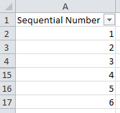
Rows 5 to 14 are hidden, but the numbers are still sequential – the formula in cell A2 has been copied down to achieve this.
The formula is
=AGGREGATE(4,5,$A$1:A1)+1
The 4 at the start of the function instructs Excel to use the MAX function in the calculation.
The 5 means to ignore hidden rows.
I have used a fixed reference on the start of the range so that it expands as it is copied down.
The AGGREGATE function finds the maximum value in the visible rows above. The +1 at the end then increments that maximum number.
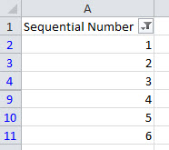
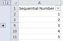
This formula will work for both filtered rows and grouped rows – see images below.
NOTE: the AGGREGATE function was added in Excel 2010 and only works on vertical ranges – it doesn’t work across columns.
Please note: I reserve the right to delete comments that are offensive or off-topic.