Hyperlinks are a great way to navigate around large spreadsheets. Unfortunately they each take a few clicks to create and can be easily broken. You can use a function to easily create multiple, flexible hyperlinks.

Excel’s HYPERLINK function provides a way to create a hyperlink based on entries in cells. This can be useful for documentation and instructions, where you can set up a table of entries to create hyperlinks.

Using the HYPERLINK function has a few requirements you need to be aware of. It is also very exacting in its requirements. Get a character wrong and the hyperlink won’t work. Using cell entries to create the hyperlink however makes it easier to tweak and correct.

Preliminaries

You will need to join text together to get the hyperlink references to work. The text joining operator is &. You use it like

=A1&B1

The above formula joins the text in A1 and B1 together – see image below.

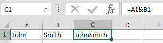Note there is no space between the names.

Current Sheet Link

To create a hyperlink to a cell in the sheet where the HYPERLINK function is used, you must include the file name, including the suffix, enclosed in square brackets (braces) followed by the cell reference.

Rather than entering the file name you can use a formula to extract the file name. It is a long formula but you can use it in any cell in any sheet, so it is easy to copy and paste into a sheet.

=MID(CELL("filename",$A$1),FIND("[",CELL("filename",$A$1)),FIND("]",CELL("filename",$A$1))-FIND("[",CELL("filename",$A$1))+1)

This places the full file name within square brackets, ready to use with the HYPERLINK function.

See the table below – this table is in the INDEX sheet in the file that can be downloaded at the bottom of this post.

Cell A2 contains the above formula.

Volatile

Just a note on using the CELL function. It is a volatile function, which means it calculates each time Excel calculates, most functions only calculate when something in the their range changes. So using thousands of CELL functions can slow down your model, though this is less of an issue with today’s fast PC’s and laptops. Rather than using the above formula multiple times, just use it once and then link to it. Cell A3 in the above table is linked to A2 and copied down.

Columns A and B in the above table are for input. Cell A2 contain A10. Cell B2 is blank. Cell E2 contains the following HYPERLINK formula that will jump to cell A10 in this sheet when you click on the word link in cell E2.

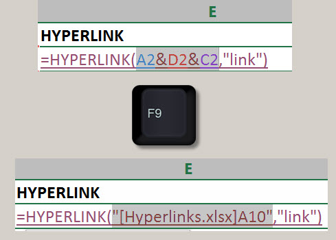
=HYPERLINK(A2&D2&C2,"link")

This formula combines three cells A2, D2 and C2 to create the required hyperlink reference. Because B2 is blank it doesn’t affect the reference created.

To see how a formula works you can select part of it in the Formula Bar and press the F9 key to see the result. The part you select must able to return a result. See image below

 

Link to Another Sheet

To link to a cell on another sheet you must include the sheet name in the reference. The trick here is that a sheet name with a space in it has a slightly different reference than a sheet name without a space.

To make it easy to refer to any sheet it is best to amend the sheet name in another cell. That’s what column D does, it converts the sheet name entered in column B into the structure used as part of the reference. The formula in cell D2 is

=IF(LEN(B2)>0,"'"&B2&"'!","")

This formula has been copied down the column in the table. The IF function basically checks the length of the cell in column B. If there are any characters in the cell, it with return TRUE and it will add a single inverted comma at the start of the sheet name and a single inverted comma at the end of the name followed by the exclamation mark (!). The ! is Excel’s identifier for a sheet name.

If the cell entry in column B is blank, the LEN function will return zero and then the IF function will return two quotation marks together, which represents a blank cell in Excel. The final reference created in cell E3 can be seen from the image below – again using F9 to display the result.

The Blank sheet name doesn’t need the single inverted commas around it to work as it doesn’t have a space in it, but including them makes no difference, the link still works. The single inverted commas are required for any sheet name that contains a space, like Month Report in row 4.

Range Name Link

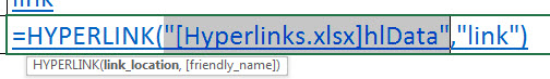
You can refer to a reference in another sheet without using the sheet name, if you use a range name. I have named cell A1 in the Data sheet. The cell is named hlData.

As you can see from the table, I have not included a sheet name in row 5. The HYPERLINK function still works – see the F9 result below of the reference created.

I tend to use prefixes for my special use range names eg hl prefix for hyperlinks. That way the names are listed together – making them easier to select when I start typing the prefix.

Creating Links

Armed with the solutions to the typical problems associated with the HYPERLINK function, you can see that using range names simplifies the process of creating hyperlinks via formulas because you don’t need the sheet name reference.

Example File below.

Hyperlinks