Excel has great charts to help you visual your numbers, but it can also allow you to use flowcharts to help visualise numbers in a different way and help explain relationships between numbers and how they are formulated.

Excel has built-in flowchart shapes, as well as other shapes. You can be creative in using these shapes and linking them to cell contents to help show how figures fit together. (The bottom of this post shows where the flowcharting options are.)

In the image below I have three values, Sales, Cost of Sales and Margin. I have used three flowchart shapes that are linked to cells.

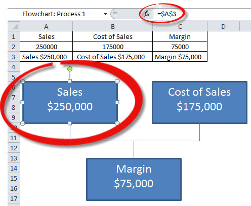
The Sales rectangle is selected and you can see the reference to cell A3 in the Formula Bar. You can only refer to a single cell in the Formula Bar when the shape is selected. Hence you need to use formulas in the linked cell to create the layout and formats you require.

To have Sales on the first line and the value on the second line you need to use a special function that inserts a line break. The formula for cell A3 which does all the work is

=A1&" "&CHAR(10)&TEXT(A2,"$#,###")

The & character joins text together. The CHAR function returns certain characters. CHAR(10) is the line break character and forces the value to appear on a separate line in the rectangle.

The TEXT function is used to format the number with $ and comma.

Cell A3 has been copied across to the other two cells B3 and C3. The other two flowchart rectangles are linked to the other two cells.

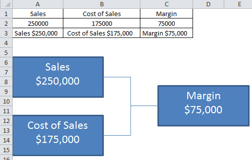
You can move the rectangles around to achieve the layout you require – see image below.

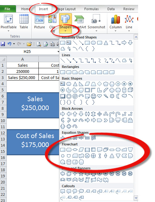
You can access the Flowchart shapes and connectors from the Insert ribbon tab and the Shapes icon – see below.

Flowchart example.